predictors may be both quantitative and categorical variables. This is based on the fact, that categorical variables may be decomposed into \(k - 1\) binary (0-1) variables (where \(k\) is number of categories/levels). In general, the maximum number of predictors is limited by degrees of freedom in the model.
Complexity of the model measured by the model number of degrees of freedom may never exceed total \(DF\) (i.e. number of observations – 1).
Models containing two or more predictors may also contain interaction terms (\(c\)):
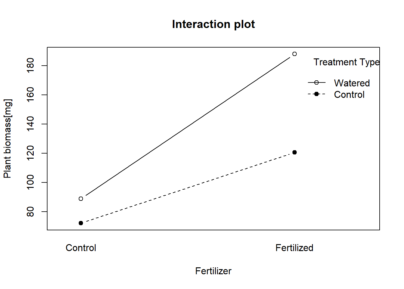
Interaction means that the dependence of the response variable on one predictor (\(X_1\)) depends on the value of second predictor (\(X_2\)). Interaction it typically tested in multi-way ANOVA, where even higher-order interactions can be considered. Interaction may be positive (i.e. the value of response is higher than expected from additive sums of main effects; in such case \(c_1 > 0\); Fig. 11.1) or negative (response value is lower that the additive sum; \(c_1 < 0\)).
The interaction is formally notated by × (Alt + 0215), i.e. \(Y \sim X_1 + X_2 + X_1 × X_2\). In R, interaction may be represented by “*” which indicates both additive and interaction effects or by “:” which indicates just the interaction term.
Note that:
testing the interaction is very common in manipulative experiments
interaction does not mean correlation between predictors
As you will see later, correlation between predictors is a serious problem which among other issues prevents from reasonable assessment of interactive effects.
Figure 1: Interaction plot showing positive interactive effects of fertilizer application and watering on plant growth. The interaction is directly visible from the graph as non-parallel lines connecting the mean values.
Testing of linear models and their terms
Statistical significance testing of linear models (as whole predictor structures) using e.g. an F-test is easy and largely follows the same principles as in simple regression. It is more difficult to decide which predictors to include in the model and which not. Finding the best model is done through a model selection procedure that aims to identify the model containing only the predictors that have a significant effect on the response, while leaving out those that are non-significant (i.e., do not contribute to the predictive power of the model). Such models are called minimum adequate models. Philosophically, they are based upon the principle of Occam’s razor or parsimony.
Statistical methods are very efficient if applied to model testing and/or comparisons between models. However, there are no universal guidelines for model/predictor selection in all cases. In models with few candidate predictors, it is possible to fit all possible models and select the one with the highest explanatory power. Frequently (but certainly not always), simple testing of the significance of individual predictors can be performed by comparing models that exclude and include the given predictor.
For efficient model selection, we need:
a measure of model quality (or quality comparison between models)
a strategy for building the model.
Measures of model quality
There are several measures of model quality or parameters of model comparison.
F-test
The F-test may not only be used to test the significance of a model but also to test whether one model is significantly better than another. Works generally well for models with up to a moderate number of observations (~200). With large n, almost all predictors tend to be significant even if they explain very little variability in the response.
R2
The proportion of explained variation is a property of the model itself. It is easy to interpret. For model comparisons, its main disadvantage is that adding more predictors always increases R2, even if the added predictor has little effect. As such, it is not suitable to compare models of different complexity.
This measure is derived from information theory and allows straighforward comparisons of model quality. Models with a lower AIC value are better. The AIC is computed using the following formula:
\[
AIC = 2k - 2log(L)
\]
where \(k\) is the number of parameters of the model and \(log(L)\) is the log-likelihood1 of the model. Essentially, AIC combines model quality (\(L\)) and complexity expressed as the number of parameters (\(k\)) into one number.
By accounting for the complexity, it also prevents the models to became overfitted (i.e. working precisely on the original data, but totally failing to predict values outside what it was trained on).
AICC
AICC is a very similar measure, which is corrected for use with small sample sizes. As a result, it is slightly more conservative, i.e. prefers model simplicity over explanatory power.
Likelihood-ratio
The likelihood ratio is a very general approach which can be used to compare many types of models. It is based on the principle that the logarithm of the likelihood ratio (which numerically equals the difference between log-likelihoods) multiplied by 2 follows the χ2 distribution; thus, the goodness-of-fit test may be used for testing models differing in numbers of degrees of freedom.
Model building strategies
Data exploration - first step
It is generally good to start with an exploratory analysis of the data to examine variable distributions and shapes of their dependencies. This is generally done by plotting a matrix of pairwise plots. Such exploratory analysis helps identify intercorrelated predictors (the inclusion of which in the candidate predictor set is problematic – see below), data transformation needs, or possible non-linear relationships. Thus, the exploratory analysis may lead to adjustments of the original dataset.
Multi-model comparisons
Then, there are several options for building a model. Theoretically, the best way would be to fit all possible models and choose the best-fitting one, e.g., based on AIC. However, the number of possible models could be very large (increasing with the number of predictors and the complexity of interaction terms), and fitting models may be demanding on computer power (even with current fast computers and the increasing availability of big data).
Still, this option is available in the function dredge() in the package MuMIn. Nevertheless, researchers are generally encouraged to use a more specific comparison between a predefined set of models, rather than the mindless comparison of everything. The comparison among models can be done by the AICtab()/AICctab() function of the package bbmle.
Stepwise model selection
Another option is the so-called stepwise selection, which can go from two different directions forward and backward. Forward selection starts with the null (intercept-only) model. Next step includes testing every model containing single predictor against the null model. Such comparisons are indicative of individual predictor explanatory power and on this basis the best fitting predictor (using R2 or AIC) can be added to the model.
In the next step the model containing the selected predictor is used as the null against with the other predictors are tested and so on until there is no significant candidate predictor left. With two or more predictors in the model, interactions between the predictors may also be tested to be included in the model.
An advantage of this approach is its intuitiveness and possibility to use a large number of candidate predictors (though multiple testing issue should be considered here). However, there are also disadvantages related with this approach including often high risk of selecting of non-optimal model due to constraints related to the procedure.
Therefore, forward selection mostly considered an outdated approach, which can and should mostly be replaced with multi-model comparisons based on AIC (see above). Still forward selection remaind a reasonable choice for observational data in multivariate models (e.g. constrained ordinations), where AIC comparisons are not available.
Backward selection uses an opposite strategy – first a saturated model is fitted (i.e., model containing all candidate predictors together with all their interactions – these may be limited up to a specified order). Non-significant terms are then removed from the model one-by-one starting with poorest predictors (measured by AIC or significance testing). Note that in the case of a significant interaction, main effects are retained in the model even if they are not significant themselves (if the same model was built-up in a forward manner, such interactions would never be tested). Backward selection is still an accepted model-building strategy for data coming from manipulative experiments. Such data typically have a limited numbers of predictors and observations, which makes them suitable to classical statistical test.
Correlation between predictors
Correlation between predictors is a serious issue in multiple regression analysis. This issue concerns observational data because in experimental studies, we should use an experimental design which ensures independence of tested predictors. The problem is, that if there are two inter-correlated candidate predictors to be included in the model, one of them may be included just by chance (because it may look slightly better with given data). The other predictor will then never be included in the model, because its effect is already accounted for by the first predictor. Depending on the actual data, either one or the other predictor may be included while the other left out.
Such inconsistency may lead to very different conclusions even if the relationships between the variables are the same and the data are just slightly different. Such cases are quite common in nature, e.g. soil pH and Ca concentration represent a common case in ecological studies. Unfortunately, none of the model building strategies or model quality measures can control this. However, a detailed exploration of the associations between the predictors themselves and between individual predictors and the response may be useful.
As a part of this exploration, we may first analyze marginal or simple effects – i.e. effects of given predictor on the response which ignore the effects of other variables. These are simple linear regressions (or one-way ANOVA) and are indicative of the correlation structure in the study system. Conversely, partial or conditional effects can be computed (i.e. unique effects of individual predictors), which are computed by testing a given predictor against a model containing all other predictors. Such effects are greatly affected by predictor inter-correlation but if significant, they may really point to mechanisms underlying the correlations.
Computing marginal and partial effects is then a part of a more general approach called variation partitioning. With this approach, you can describe the correlation structure among the predictors (or frequently groups of predictors) and quantify their unique or shared effects on the response variable.
NoteHow to do in R
1. Explanatory analysis
Pair plots showing correlation between variables can be done by ggpairs() from the package Ggally, or pairs.panels() from the package psych.
2. Fitting a model
Function lm(). Individual predictors are included in the formula on the predictor side separated, by + (additive effects) or by * (both, additive and interactive effects).
3. Forward selection or simple effects
Testing candidate predictors to be included in the model is done by function add1() in forward selection:
Parameter test is then used for the specification of the model quality criterion. AIC is displayed always; for ordinary linear models, it makes sense to ask for an F-test by setting test = "F".
add1() can also be used for testing predictor simple effects.
4. Backward selection
Testing predictors to be removed from the model can be done using function drop1(). The use is similar to add1(), just the parameter scope is not specified.
5. Changing model structure
Function update() adds or removes a predictor from a model (“manually”).
update() can be used to change other parameters of a model aswell.
6. Comparison of model quality
Function anova() (e.g. anova(model1, model2)) compares model2 vs model1 by AIC.
7. Model comparisons
AICtab(), AICctab() from the package bbmle provide comparisons of model quality by AIC/AICC. Compared models are simply listed as arguments of the function. You have to prepare a set of candidate models yourself.
dredge() of the package MuMIn fits all models defined by all possible subsets of the provided full model and compares them by AIC/AICC.
8. Testing individual terms
anova(lm.model) displays sequential F-tests for individual terms. Sequential testing means that the order of the predictors affects the results (unless the predictors are perfectly independent - orthogonal).
summary(lm.model) displays detailed model statistics - F-test of the whole model and t-tests of individual regression coefficients. These t-tests are not sequential and thus are independent of the term order in the model.
9. Model coefficients
Function coef() shows model coefficients.
10. Model residuals
Function resid() displays model residuals.
11. Extraxt fitted values
Fitted (predicted) values can be obtained with the predict_response() function of the package ggeffects. This can be plotted directly with ggplot.
Exercises
Data are availabe in separate Excel sheets.
The number of seedlings per square meter was monitored at 24 grasslands, which were mown once (mown1), mown twice (mown2), or grazed (variable treatment). In addition, biomass production was measured together with the mean annual temperature of each grassland. Build a multiple regression model predicting the effects of grassland parameters on seedling density.
Transpiration of plants was recorded together with air humidity, temperature, wind speed, and sunny vs. cloudy weather. On which of these variables does the transpiration rate depend?
The effect of watering and fertiliser application on plant growth (measured by biomass production) was tested in the full-factorial manipulative experiment. Perform a two-way analysis of variance and test the interaction between the two treatments.
The effect of physical exercise and diet on body mass was studied in 21 people. In addition to the studied variables, body height, hair color, and sex were also recorded as presumed important covariates. What does the body mass depend on?
Real data tasks
Analyse the dependence between vegetation species richness (=number of species) and all predictors describing soil properties and past management in the dataset of vegetation plots of Latvian grasslands. Consider appropriate transformations of the data if needed. The data are available from data/LatviaGrasslands.xlsx The data come from the master thesis of Martin Franc (in Czech with English abstract).
#AI Ask your favourite LLM to solve any of the tasks and generate the corresponding R script. Compare the LLM solution with yours
Footnotes
The likelihood is something as “accuracy score” measuring how well the model actually explains the data, i.e. how much do its predictions match the reality. And why log? Well, this is mainly practical - the the chance (likelihood) that the model will predict every single data point right is very very small (e.g., 0.00000000000000000001) and as you can imagine, working with such numbers is a nightmare. For this purpose, we use the log(L), where the terrible number suddenly looks like this: -46.0517.↩︎