library(tidyverse)
library(readxl)
library(janitor)5 Join Functions
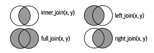
In this chapter, we will learn how to merge information from another dataset (using left_join(), full_join()) and how to filter our data based on another dataset (semi_join(), anti_join()). We will also utilise our skills from the previous chapter to calculate various statistics about our data, such as mean indicator values, community-weighted means of certain traits, and the proportion of specific plant groups (using left_join(), group_by(), and summarise()). We will also use mutate() with additional conditions (ifelse(), case_when()).
Credits: https://r4ds.hadley.nz/joins.html
5.1 Matching selected information with left_join()
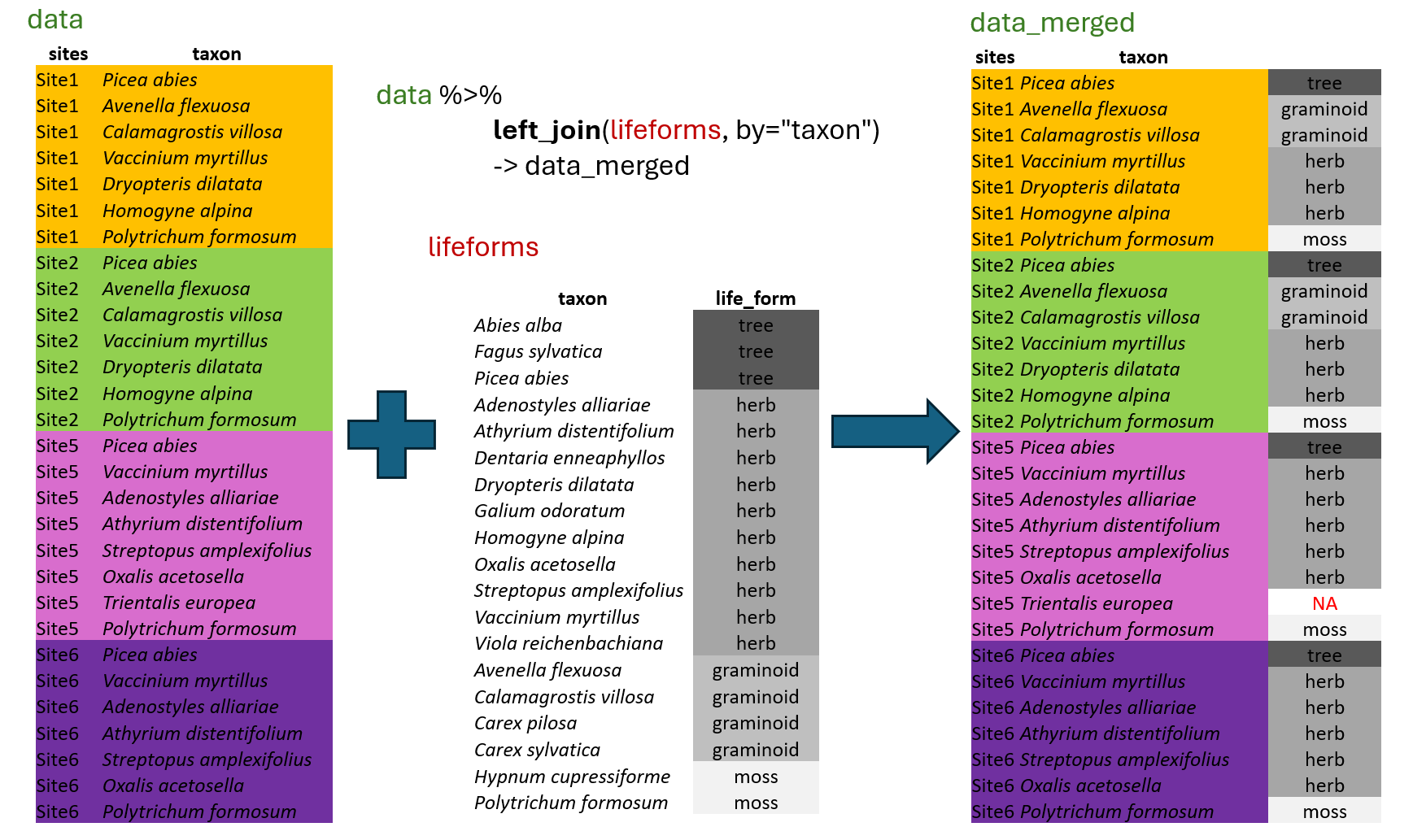
In most cases, the data you need for analyses is not organised in one file, but rather in multiple files. For example, we have measured characteristics, known as traits, for each species in the region, and we have species lists for all the sites. To calculate the mean values of selected traits for each site, we must first append the information to individual records. For this, we will use the function called left_join(), which belongs to the group of mutating joins available in the tidyverse package dplyr.
 This function will automatically look for columns with exactly matching names, or we can specify the corresponding variables directly using the
 by argument. It will append all the columns available in the second “lifeforms” dataset, but only for rows where there is an exact match. Although we have information for other species, such as Abies alba or Carex sylvatica, these do not have matching rows in the first dataset, “data”, and the information will therefore not be used. This means that left_join() is only selecting rows that are present in the first dataset. If the information is missing in the matching file, for example, if there is no information for Trientalis europaea in the lifeforms dataset, the resulting file will contain NA.
Let’s train a bit. Start a new script for this chapter again.
We will import the data from the Forest understory again.
spe <- read_xlsx("data/forest_understory/Axmanova-Forest-spe.xlsx")We will also import data with some traits, such as plant height and Ellenberg-type indicator values, which indicate demands on environmental factors, including soil reaction, light, and nutrients. Lower values indicate lower demands, meaning that species can tolerate low (acidic) pH levels or low nutrient levels. High values suggest that the species requires or grows in habitats with high (basic) soil reaction and high nutrient availability.
traits <- read_xlsx("data/forest_understory/traits.xlsx")If we try to merge these two files directly, it does not work. We will get a warning explaining that there are no common variables.
spe %>% left_join(traits)Error in `left_join()`:
! `by` must be supplied when `x` and `y` have no common variables.
ℹ Use `cross_join()` to perform a cross-join.So there are more options for what we can do. We verify the data and find that the required information to match is stored once as ‘Species’ (in the data) and once as ‘Taxon’ (in traits).
tibble(spe)# A tibble: 2,277 × 4
RELEVE_NR Species Layer CoverPerc
<dbl> <chr> <dbl> <dbl>
1 1 Quercus petraea agg. 1 63
2 1 Acer campestre 1 18
3 1 Crataegus laevigata 4 2
4 1 Cornus mas 4 8
5 1 Lonicera xylosteum 4 3
6 1 Galium sylvaticum 6 3
7 1 Carex digitata 6 3
8 1 Melica nutans 6 2
9 1 Polygonatum odoratum 6 2
10 1 Geum urbanum 6 2
# ℹ 2,267 more rowstibble(traits)# A tibble: 316 × 7
Taxon Height SeedMass EIV_Light EIV_Moisture EIV_Reaction EIV_Nutrients
<chr> <dbl> <dbl> <dbl> <dbl> <dbl> <dbl>
1 Quercus pe… 25 975. 6 5 5 4
2 Acer campe… 7.5 54.3 5 5 7 6
3 Crataegus … 5.5 276. 5 5 7 5
4 Cornus mas 4 488. 6 4 8 5
5 Lonicera x… 2 164. 4 5 7 6
6 Galium syl… 0.85 1.10 5 5 6 5
7 Carex digi… 0.2 1.44 4 5 6 6
8 Melica nut… 0.45 2.49 4 5 6 4
9 Polygonatu… 0.45 264. 6 3 7 3
10 Geum urban… 0.55 2.05 5 5 6 7
# ℹ 306 more rowsWe can decide to rename the ‘Species’ column to ‘Taxon’ and use this column for matching.
spe %>% rename(Taxon = Species) %>%
  left_join(traits, by = "Taxon")
# A tibble: 2,277 × 10
RELEVE_NR Taxon Layer CoverPerc Height SeedMass EIV_Light EIV_Moisture
<dbl> <chr> <dbl> <dbl> <dbl> <dbl> <dbl> <dbl>
1 1 Quercus pet… 1 63 25 975. 6 5
2 1 Acer campes… 1 18 7.5 54.3 5 5
3 1 Crataegus l… 4 2 5.5 276. 5 5
4 1 Cornus mas 4 8 4 488. 6 4
5 1 Lonicera xy… 4 3 2 164. 4 5
6 1 Galium sylv… 6 3 0.85 1.10 5 5
7 1 Carex digit… 6 3 0.2 1.44 4 5
8 1 Melica nuta… 6 2 0.45 2.49 4 5
9 1 Polygonatum… 6 2 0.45 264. 6 3
10 1 Geum urbanum 6 2 0.55 2.05 5 5
# ℹ 2,267 more rows
# ℹ 2 more variables: EIV_Reaction <dbl>, EIV_Nutrients <dbl>Or we can even skip the by argument, as there is only one common matching column.
spe %>% rename(Taxon = Species) %>%
  left_join(traits)
Joining with `by = join_by(Taxon)`# A tibble: 2,277 × 10
RELEVE_NR Taxon Layer CoverPerc Height SeedMass EIV_Light EIV_Moisture
<dbl> <chr> <dbl> <dbl> <dbl> <dbl> <dbl> <dbl>
1 1 Quercus pet… 1 63 25 975. 6 5
2 1 Acer campes… 1 18 7.5 54.3 5 5
3 1 Crataegus l… 4 2 5.5 276. 5 5
4 1 Cornus mas 4 8 4 488. 6 4
5 1 Lonicera xy… 4 3 2 164. 4 5
6 1 Galium sylv… 6 3 0.85 1.10 5 5
7 1 Carex digit… 6 3 0.2 1.44 4 5
8 1 Melica nuta… 6 2 0.45 2.49 4 5
9 1 Polygonatum… 6 2 0.45 264. 6 3
10 1 Geum urbanum 6 2 0.55 2.05 5 5
# ℹ 2,267 more rows
# ℹ 2 more variables: EIV_Reaction <dbl>, EIV_Nutrients <dbl>We can also skip the rename() step and directly say in the left_join() function what is matching with what. Note that it will retain ‘Species’ as the outcome, because this was how we named it in the primary data file.
spe %>% left_join(traits, by = c("Species" = "Taxon"))# A tibble: 2,277 × 10
RELEVE_NR Species Layer CoverPerc Height SeedMass EIV_Light EIV_Moisture
<dbl> <chr> <dbl> <dbl> <dbl> <dbl> <dbl> <dbl>
1 1 Quercus pet… 1 63 25 975. 6 5
2 1 Acer campes… 1 18 7.5 54.3 5 5
3 1 Crataegus l… 4 2 5.5 276. 5 5
4 1 Cornus mas 4 8 4 488. 6 4
5 1 Lonicera xy… 4 3 2 164. 4 5
6 1 Galium sylv… 6 3 0.85 1.10 5 5
7 1 Carex digit… 6 3 0.2 1.44 4 5
8 1 Melica nuta… 6 2 0.45 2.49 4 5
9 1 Polygonatum… 6 2 0.45 264. 6 3
10 1 Geum urbanum 6 2 0.55 2.05 5 5
# ℹ 2,267 more rows
# ℹ 2 more variables: EIV_Reaction <dbl>, EIV_Nutrients <dbl>Note that left_join() is a great help. However, you should always consider the data. If you have more potentially matching rows, you can create a lot of unwanted mess with left_join(). For example, if you do not use a unique ID, but a descriptor such as forest type. Please read the warning messages carefully. :-)
5.2 full_join() vs. bind_rows()
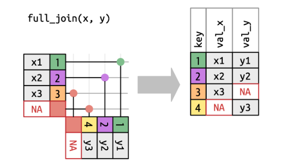
Sometimes it is needed to match both datasets. In contrast to left_join(), full_join() will also add additional rows that appear in the other dataset.
Credits: https://r4ds.hadley.nz/joins.html
We will upload the forest env data and make two subsets to train a bit.
env <- read_xlsx("data/forest_understory/Axmanova-Forest-env.xlsx")In the first subset, we will use only the first two forest types, namely oak and oak-hornbeam forests and the selection of variables.
forest1 <- env %>% filter(ForestType %in% c(1, 2)) %>%
  select(PlotID = RELEVE_NR, ForestType, ForestTypeName, pH_KCl, Biomass)
In the second subset, we will use one forest type shared with the previous subset and two others: oak-hornbeam, ravine, and alluvial forests, with a slightly different selection of variables.
forest2 <- env %>%
  filter(ForestType %in% c(2, 3, 4))%>%
  select(PlotID = RELEVE_NR, ForestType, ForestTypeName, pH_KCl, Canopy_E3)
Now, left_join() the data and check the preview (use view()) to see more of the dataset. We have added the extra information available in the second dataset to our selection of plots and variables in the first dataset.
forest1 %>%
  left_join(forest2)
Joining with `by = join_by(PlotID, ForestType, ForestTypeName, pH_KCl)`# A tibble: 44 × 6
PlotID ForestType ForestTypeName pH_KCl Biomass Canopy_E3
<dbl> <dbl> <chr> <dbl> <dbl> <dbl>
1 1 2 oak hornbeam forest 5.28 12.8 80
2 2 1 oak forest 3.24 9.9 NA
3 3 1 oak forest 4.01 15.2 NA
4 4 1 oak forest 3.76 16 NA
5 5 1 oak forest 3.50 20.7 NA
6 6 1 oak forest 3.8 46.4 NA
7 7 1 oak forest 3.48 49.2 NA
8 8 2 oak hornbeam forest 3.68 48.7 85
9 9 2 oak hornbeam forest 4.24 13.8 80
10 10 1 oak forest 4.00 79.1 NA
# ℹ 34 more rowsIn the next step, we will combine both subsets using a full_join(). What is the output? We will obtain a dataset containing all available information, encompassing all four forest types. However, since Forest type 1 is only present in the first subset, the corresponding rows will include only the information available there (forest type and pH). The Type 2 is present in both datasets so that it will contain all information from both datasets (forest type, pH, biomass, and canopy). Types 3 and 4 will have information only from the second dataset (forest type, pH, canopy). Use view() to see the complete merged dataset.
forest1 %>%
  full_join(forest2)
Joining with `by = join_by(PlotID, ForestType, ForestTypeName, pH_KCl)`# A tibble: 65 × 6
PlotID ForestType ForestTypeName pH_KCl Biomass Canopy_E3
<dbl> <dbl> <chr> <dbl> <dbl> <dbl>
1 1 2 oak hornbeam forest 5.28 12.8 80
2 2 1 oak forest 3.24 9.9 NA
3 3 1 oak forest 4.01 15.2 NA
4 4 1 oak forest 3.76 16 NA
5 5 1 oak forest 3.50 20.7 NA
6 6 1 oak forest 3.8 46.4 NA
7 7 1 oak forest 3.48 49.2 NA
8 8 2 oak hornbeam forest 3.68 48.7 85
9 9 2 oak hornbeam forest 4.24 13.8 80
10 10 1 oak forest 4.00 79.1 NA
# ℹ 55 more rowsNote that the joining worked well, since we had the same names in both datasets. For example, if biomass were called soil_pH in one and pH_KCl in the other dataset, it will treat them as different variables, as you can see below:
forest1 %>%
  rename(soil_pH = pH_KCl) %>%
  full_join(forest2)
Joining with `by = join_by(PlotID, ForestType, ForestTypeName)`# A tibble: 65 × 7
PlotID ForestType ForestTypeName soil_pH Biomass pH_KCl Canopy_E3
<dbl> <dbl> <chr> <dbl> <dbl> <dbl> <dbl>
1 1 2 oak hornbeam forest 5.28 12.8 5.28 80
2 2 1 oak forest 3.24 9.9 NA NA
3 3 1 oak forest 4.01 15.2 NA NA
4 4 1 oak forest 3.76 16 NA NA
5 5 1 oak forest 3.50 20.7 NA NA
6 6 1 oak forest 3.8 46.4 NA NA
7 7 1 oak forest 3.48 49.2 NA NA
8 8 2 oak hornbeam forest 3.68 48.7 3.68 85
9 9 2 oak hornbeam forest 4.24 13.8 4.24 80
10 10 1 oak forest 4.00 79.1 NA NA
# ℹ 55 more rows*Tip: if you are merging data from different sources and you get a similar mess, check the function coalesce() https://dplyr.tidyverse.org/reference/coalesce.html.
Imagine a situation where data were sampled in different years/months or by different colleagues, or in different regions separately. If these subsets have exactly the same structure, we can use the bind_rows() function to merge them, one below the other.
forest1 <- env %>%
  filter(ForestType == 1) %>%
  select(PlotID = RELEVE_NR, ForestType, ForestTypeName, pH_KCl, Biomass)

forest2 <- env %>%
  filter(ForestType == 2)%>%
  select(PlotID = RELEVE_NR, ForestType, ForestTypeName, pH_KCl, Biomass)
Bind and check the whole dataset with view().
forest1 %>%
  bind_rows(forest2)
# A tibble: 44 × 5
PlotID ForestType ForestTypeName pH_KCl Biomass
<dbl> <dbl> <chr> <dbl> <dbl>
1 2 1 oak forest 3.24 9.9
2 3 1 oak forest 4.01 15.2
3 4 1 oak forest 3.76 16
4 5 1 oak forest 3.50 20.7
5 6 1 oak forest 3.8 46.4
6 7 1 oak forest 3.48 49.2
7 10 1 oak forest 4.00 79.1
8 11 1 oak forest 3.83 7.4
9 28 1 oak forest 3.56 29.7
10 31 1 oak forest 3.20 14.9
# ℹ 34 more rowsNote that the rbind() function in base R works similarly, but less effectively and it is designed for data frames.
rm(forest1, forest2) #remove unwanted data from the environment5.3 Filtering joins
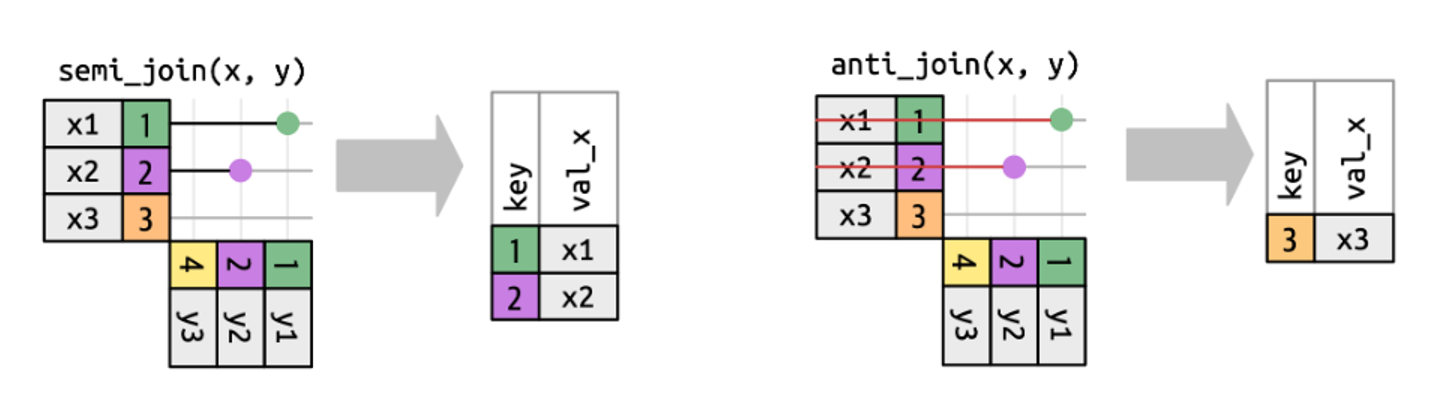
Sometimes we need to filter the data according to another dataset. For example, we have reviewed the environmental file and determined that for a follow-up analysis, we only need the alluvial forest data. Therefore, we filtered rows in the env file.
env_selected <- env %>%
  filter(ForestType == 4)%>%
  select(PlotID = RELEVE_NR,ForestType, ForestTypeName, pH_KCl, Biomass) %>%
  print()
# A tibble: 11 × 5
PlotID ForestType ForestTypeName pH_KCl Biomass
<dbl> <dbl> <chr> <dbl> <dbl>
1 101 4 alluvial forest 6.67 91.1
2 103 4 alluvial forest 7.12 114.
3 104 4 alluvial forest 7.14 188.
4 110 4 alluvial forest 5.82 126.
5 111 4 alluvial forest 7.01 84.8
6 113 4 alluvial forest 6.61 74.5
7 125 4 alluvial forest 4.99 123.
8 128 4 alluvial forest 7.03 121.
9 130 4 alluvial forest 5.74 238
10 132 4 alluvial forest 5.56 287.
11 127 4 alluvial forest 5.56 176 However, we also need to filter the rows in the species data where there is no information about forest types. The only common identifier is the PlotID (i.e. sample/site ID).
spe %>% rename(PlotID = RELEVE_NR) %>%
  semi_join(env_selected)
Joining with `by = join_by(PlotID)`# A tibble: 530 × 4
PlotID Species Layer CoverPerc
<dbl> <chr> <dbl> <dbl>
1 101 Fraxinus excelsior 1 38
2 103 Alnus glutinosa 1 63
3 104 Alnus glutinosa 1 63
4 110 Alnus glutinosa 1 38
5 111 Alnus glutinosa 1 38
6 113 Alnus glutinosa 1 63
7 125 Alnus glutinosa 1 38
8 128 Corylus avellana 1 38
9 130 Acer pseudoplatanus 1 38
10 132 Alnus glutinosa 1 38
# ℹ 520 more rowsWith the distinct() function, you can check if the IDs are the same.
spe %>% rename(PlotID = RELEVE_NR) %>%
  semi_join(env_selected) %>%
  distinct(PlotID)
Joining with `by = join_by(PlotID)`# A tibble: 11 × 1
PlotID
<dbl>
1 101
2 103
3 104
4 110
5 111
6 113
7 125
8 128
9 130
10 132
11 127Sometimes you may need the opposite - to keep only rows/IDs that are not in the other file. For this, you should use the anti_join() function. For example, you may want to remove a particular group of species from your list, such as annuals or non-vascular plants (mosses and lichens).
5.4 Advanced mutate() and .by
Below are a few examples of how we used mutate() so far
env %>%
  mutate(author = "Axmanova", #add one column with specified value
        forestType = as.character(ForestType), #change the type of variable
        biomass = Biomass * 1000, # multiply to change to mg
        forestTypeName = str_replace_all(ForestTypeName, " ", "_")) %>% #change string
  select(PlotID = RELEVE_NR, author, forestType, biomass, forestTypeName)
# A tibble: 65 × 5
PlotID author forestType biomass forestTypeName
<dbl> <chr> <chr> <dbl> <chr>
1 1 Axmanova 2 12800 oak_hornbeam_forest
2 2 Axmanova 1 9900 oak_forest
3 3 Axmanova 1 15200 oak_forest
4 4 Axmanova 1 16000 oak_forest
5 5 Axmanova 1 20700 oak_forest
6 6 Axmanova 1 46400 oak_forest
7 7 Axmanova 1 49200 oak_forest
8 8 Axmanova 2 48700 oak_hornbeam_forest
9 9 Axmanova 2 13800 oak_hornbeam_forest
10 10 Axmanova 1 79100 oak_forest
# ℹ 55 more rowsWe also used mutate() to adjust more variables at once:
env %>% mutate(across(c(Radiation, Heat), ~ round(.x, digits = 2))) %>%
  select(PlotID = RELEVE_NR, Radiation, Heat)
# A tibble: 65 × 3
PlotID Radiation Heat
<dbl> <dbl> <dbl>
1 1 0.88 0.86
2 2 0.93 0.81
3 3 0.92 0.85
4 4 0.93 0.95
5 5 0.87 0.87
6 6 0.92 0.88
7 7 0.83 0.8
8 8 0.87 0.87
9 9 0.61 0.42
10 10 0.91 0.93
# ℹ 55 more rows.x refers to the entire column (vector) being transformed inside a function like mutate(across(...)) or map().
Alternatively, if you have a large table with only measured variables, you can specify what should not be used, here Species, and mutate() will be applied to everything left. This is especially useful for changing formats, e.g., from character to numeric (using the function as.numeric()).
iris %>%
  as_tibble() %>%  #first change from dataframe to tibble
  mutate(across(-Species,~round(.x, digits = 1)))
# A tibble: 150 × 5
Sepal.Length Sepal.Width Petal.Length Petal.Width Species
<dbl> <dbl> <dbl> <dbl> <fct>
1 5.1 3.5 1.4 0.2 setosa
2 4.9 3 1.4 0.2 setosa
3 4.7 3.2 1.3 0.2 setosa
4 4.6 3.1 1.5 0.2 setosa
5 5 3.6 1.4 0.2 setosa
6 5.4 3.9 1.7 0.4 setosa
7 4.6 3.4 1.4 0.3 setosa
8 5 3.4 1.5 0.2 setosa
9 4.4 2.9 1.4 0.2 setosa
10 4.9 3.1 1.5 0.1 setosa
# ℹ 140 more rowsYou can even create a list of functions which should be applied. The relocate() function was used here to shift all the Sepal variables before the first variable (just for an easier check).
iris%>%
  as_tibble() %>%
  mutate(across(starts_with("Sepal"),
                list(rounded = round, log = log1p))) %>%
  relocate(starts_with("Sepal"), .before = 1)
# A tibble: 150 × 9
Sepal.Length Sepal.Width Sepal.Length_rounded Sepal.Length_log
<dbl> <dbl> <dbl> <dbl>
1 5.1 3.5 5 1.81
2 4.9 3 5 1.77
3 4.7 3.2 5 1.74
4 4.6 3.1 5 1.72
5 5 3.6 5 1.79
6 5.4 3.9 5 1.86
7 4.6 3.4 5 1.72
8 5 3.4 5 1.79
9 4.4 2.9 4 1.69
10 4.9 3.1 5 1.77
# ℹ 140 more rows
# ℹ 5 more variables: Sepal.Width_rounded <dbl>, Sepal.Width_log <dbl>,
# Petal.Length <dbl>, Petal.Width <dbl>, Species <fct>We can further mutate a variable using the group_by() function. This can be illustrated step by step, as shown below…
env %>%
  group_by(ForestType) %>%
  select(PlotID = RELEVE_NR, ForestType, Biomass) %>%
  mutate(meanBiomass = mean(Biomass)) %>%
  mutate(comparison = (case_when(Biomass > meanBiomass ~ "higher",
                               Biomass < meanBiomass ~ "lower",
                               TRUE ~ "equal"))) %>%
  arrange(ForestType, desc(Biomass))
# A tibble: 65 × 5
# Groups: ForestType [4]
PlotID ForestType Biomass meanBiomass comparison
<dbl> <dbl> <dbl> <dbl> <chr>
1 10 1 79.1 26.7 higher
2 7 1 49.2 26.7 higher
3 6 1 46.4 26.7 higher
4 44 1 34.1 26.7 higher
5 82 1 33.9 26.7 higher
6 28 1 29.7 26.7 higher
7 42 1 21.5 26.7 lower
8 5 1 20.7 26.7 lower
9 81 1 20.6 26.7 lower
10 4 1 16 26.7 lower
# ℹ 55 more rowsOr like this, where we do not use a standalone group_by() but rather include it directly in the mutate() function with the .by argument.
env %>%
  select(PlotID=RELEVE_NR, ForestType, Biomass)%>%
  mutate(
    meanBiomass = mean(Biomass, na.rm = TRUE),
    comparison = case_when(
      Biomass > meanBiomass ~ "higher",
      Biomass < meanBiomass ~ "lower",
      TRUE ~ "equal"),
    .by = ForestType)
# A tibble: 65 × 5
PlotID ForestType Biomass meanBiomass comparison
<dbl> <dbl> <dbl> <dbl> <chr>
1 1 2 12.8 44.4 lower
2 2 1 9.9 26.7 lower
3 3 1 15.2 26.7 lower
4 4 1 16 26.7 lower
5 5 1 20.7 26.7 lower
6 6 1 46.4 26.7 higher
7 7 1 49.2 26.7 higher
8 8 2 48.7 44.4 higher
9 9 2 13.8 44.4 lower
10 10 1 79.1 26.7 higher
# ℹ 55 more rowsWe need to realise that after you use group_by(), the data stay grouped until you explicitly call ungroup(), or use a verb that drops grouping automatically by default settings (usually summarise() or count()). While the summarise() removes the grouping, mutate() does not. Therefore, grouping still applies until the end of that call.
The advantage of .by is that it works only within the mutate() function.
5.5 Advanced summarise()
summarise() reduces the information to a single value per group, as defined by the group_by() function. We also used the summarise() function with across() and calculated the minimum, mean, median, maximum values, or the sum of the values.
env %>%
  group_by(ForestTypeName) %>%
  summarise(meanBiomass = mean(Biomass))
# A tibble: 4 × 2
ForestTypeName meanBiomass
<chr> <dbl>
1 alluvial forest 148.
2 oak forest 26.7
3 oak hornbeam forest 44.4
4 ravine forest 79.1We have not yet explained the n_distinct() function. It can be used for getting unique combinations of selected variables directly in summarise(). Like here, a unique number of species in each plot:
spe %>%
  summarise(unique_species = n_distinct(Species), .by = RELEVE_NR)
# A tibble: 65 × 2
RELEVE_NR unique_species
<dbl> <int>
1 1 42
2 2 16
3 3 15
4 4 20
5 5 14
6 6 19
7 7 22
8 8 23
9 9 22
10 10 18
# ℹ 55 more rowsOr unique pairs or combinations of selected variables, such as species + vegetation layers in which they appeared across the whole dataset.
spe %>%
  summarise(unique_species_layer = n_distinct(interaction(Species, Layer)))
# A tibble: 1 × 1
unique_species_layer
<int>
1 369When you become confident with joins and summarise(), you can even do something like this: We are working with env data, but at the same time, we want to use the summarised information from species data. We can calculate it directly in the pipeline without stepping outside, as there is no need to calculate and save intermediate steps separately.
env %>%
  left_join(spe %>%
              group_by(RELEVE_NR) %>%
              count(name = "Richness")) %>%
  select(PlotID = RELEVE_NR, ForestType, ForestTypeName, Richness, Biomass, pH_KCl)
Joining with `by = join_by(RELEVE_NR)`# A tibble: 65 × 6
PlotID ForestType ForestTypeName Richness Biomass pH_KCl
<dbl> <dbl> <chr> <int> <dbl> <dbl>
1 1 2 oak hornbeam forest 44 12.8 5.28
2 2 1 oak forest 17 9.9 3.24
3 3 1 oak forest 16 15.2 4.01
4 4 1 oak forest 22 16 3.76
5 5 1 oak forest 15 20.7 3.50
6 6 1 oak forest 22 46.4 3.8
7 7 1 oak forest 23 49.2 3.48
8 8 2 oak hornbeam forest 24 48.7 3.68
9 9 2 oak hornbeam forest 28 13.8 4.24
10 10 1 oak forest 19 79.1 4.00
# ℹ 55 more rowsAnother useful thing is knowing how to sum values across multiple columns and save the result in another column, i.e., row-wise sum. The relevant function is called rowSums(). We will examine the example of frozen fauna data availability. First, we will transform the table into a tidy format by filling in the 0s and changing the x value to 1.
Alternative is mutate(across(c(pollen_spores, macrofossils, dna), ~ if_else(!is.na(.x) & .x == "x", 1, 0))).
data <- read_xlsx("data/frozen_fauna/FrozenFauna_metadata.xlsx", sheet = 1) %>%
  clean_names() %>%
  mutate(across(c(pollen_spores, macrofossils, dna), ~ replace_na(.x, "0"))) %>%
  mutate(across(c(pollen_spores, macrofossils, dna), ~ if_else(.x == "x", 1, 0))) %>%
  mutate(dataAvailableSum = rowSums(across(pollen_spores:dna))) %>%
  print()
# A tibble: 27 × 7
id code species pollen_spores macrofossils dna dataAvailableSum
<dbl> <chr> <chr> <dbl> <dbl> <dbl> <dbl>
1 1 D-M5 Mammuthus pri… 0 0 1 1
2 2 D-BP4 Bison priscus 0 0 1 1
3 3 D-MP11 Mammuthus pri… 1 1 0 2
4 4 SK2 Stephanorhinu… 0 1 0 1
5 5 MP5 Mammuthus pri… 1 1 0 2
6 6 CA2 Coelodonta an… 0 1 0 1
7 7 MP9 Mammuthus pri… 1 1 1 3
8 8 D-MP10 Mammuthus pri… 1 1 0 2
9 9 MP3 Mammuthus pri… 1 1 0 2
10 10 MP4 Mammuthus pri… 1 1 0 2
# ℹ 17 more rowssummarise() is often used for obtaining so-called community means or community-weighted means. For example, we have traits for individual species, and we want to calculate a mean for each site and compare it.
spe %>%
  left_join(traits, by = c("Species" = "Taxon")) %>%
  summarise(meanHeight = mean(Height), .by = RELEVE_NR)
# A tibble: 65 × 2
RELEVE_NR meanHeight
<dbl> <dbl>
1 1 NA
2 2 6.00
3 3 3.50
4 4 8.14
5 5 3.82
6 6 NA
7 7 NA
8 8 3.52
9 9 8.25
10 10 NA
# ℹ 55 more rowsSo far, we have had data with no missing values, but you will most likely encounter situations where there are some NAs. For this, you will need to use the argument na.rm = TRUE, which indicates that you want to skip the NAs from counting. Otherwise, a single NA would mean that the result will also be NA. The same issue occurred here, so we need to address it.
spe %>%
  left_join(traits, by = c("Species" = "Taxon")) %>%
  summarise(meanHeight = mean(Height, na.rm = T), .by = RELEVE_NR)
# A tibble: 65 × 2
RELEVE_NR meanHeight
<dbl> <dbl>
1 1 4.60
2 2 6.00
3 3 3.50
4 4 8.14
5 5 3.82
6 6 3.3
7 7 4.25
8 8 3.52
9 9 8.25
10 10 3.53
# ℹ 55 more rowsWe can also consider using abundance to weight the result. This is called the community-weighted mean, and it assigns higher importance to species that are more abundant and lower importance to those that are rare. Here, the abundance is approximated as a percentage cover in the plot.
spe %>%
  left_join(traits, by = c("Species" = "Taxon")) %>%
  summarise(meanHeight = mean(Height, na.rm = T),
            meanHeight_weighted = weighted.mean(Height, CoverPerc, na.rm = TRUE),
            .by = RELEVE_NR)
# A tibble: 65 × 3
RELEVE_NR meanHeight meanHeight_weighted
<dbl> <dbl> <dbl>
1 1 4.60 12.9
2 2 6.00 16.3
3 3 3.50 16.7
4 4 8.14 17.2
5 5 3.82 15.3
6 6 3.3 9.36
7 7 4.25 12.9
8 8 3.52 11.2
9 9 8.25 14.6
10 10 3.53 14.9
# ℹ 55 more rowsYou can see that the results are pretty different! Note that we are in a forest, so we now compare the heights of the dominant trees and the smaller, less abundant herbs. Especially for the CWM, it plays a huge role. Therefore, we will now calculate the CWM only for the herb-layer (6).
spe %>%
  left_join(traits, by = c("Species" = "Taxon")) %>%
  filter(Layer == 6) %>%
  summarise(meanHeight = mean(Height, na.rm = T),
            meanHeight_weighted = weighted.mean(Height, CoverPerc, na.rm = TRUE),
            .by = RELEVE_NR)
# A tibble: 65 × 3
RELEVE_NR meanHeight meanHeight_weighted
<dbl> <dbl> <dbl>
1 1 0.379 0.367
2 2 0.496 0.483
3 3 0.430 0.404
4 4 0.598 0.593
5 5 0.563 0.527
6 6 0.562 0.561
7 7 0.491 0.522
8 8 0.452 0.657
9 9 0.492 0.481
10 10 0.539 0.555
# ℹ 55 more rowsSimilarly, we can calculate community means across multiple variables simultaneously. Here, we will try the Ellenberg-type indicator values (abbreviated as EIV), which measure species demands for particular factors. The higher the value, the higher the demands or affinity to habitats with higher values of these environmental factors. We will apply them solely based on the presence of species; no weights will be used. Therefore, we do not need to care that much about the differences among layers. However, we will keep each species only once (a list of unique species for each plot), so we will remove information about layers first and use distinct(). An alternative is to add filter(Layer == 6) %>% if we want to focus on the herb layer only.
spe %>%
  left_join(traits, by = c("Species" = "Taxon")) %>%
  select(-c(Layer, CoverPerc)) %>%
  distinct() %>%
  group_by(RELEVE_NR) %>%
  summarise(across(starts_with("EIV"), ~mean(.x, na.rm = TRUE)))
# A tibble: 65 × 5
RELEVE_NR EIV_Light EIV_Moisture EIV_Reaction EIV_Nutrients
<dbl> <dbl> <dbl> <dbl> <dbl>
1 1 5.08 4.64 6.54 4.95
2 2 4.88 4.81 4.94 4.31
3 3 4.87 4.8 4.93 4.4
4 4 5.3 4.5 5.7 4.25
5 5 6.07 4.14 5.57 3.86
6 6 5.72 4.5 6.39 5.22
7 7 5.8 4.4 6.25 4.9
8 8 5.17 4.61 5.43 4.65
9 9 5.32 4.5 5.77 4.41
10 10 6.38 3.69 6.19 3.88
# ℹ 55 more rows5.6 Exercises
1. Do a bit more with Forest understory data. Upload the env file called Axmanova-Forest-env.xlsx, create two subsets: forest1, where you select PlotID = RELEVE_NR, ForestType, ForestTypeName and forest2, with columns ForestType, pH_KCl, Biomass. Now use left_join() to match forest2 to forest1. What happened? Check how many times there are rows with the same PlotID using some simple functions.
2. Upload the data from the Lepidoptera folder. First, load the env data and check its structure. The structure is inverted, so we will first transpose it to work with it normally.
env <- read_xlsx("data/lepidoptera/env_char_MSVejnoha.xlsx") %>%
  column_to_rownames(var = "Site") %>%  # move 'Site' column to row names
  t() %>%                               # transpose like Excel
  as.data.frame() %>%                   # back to data frame
  rownames_to_column(var = "Site") %>%  # make the row names a column again
  as_tibble() %>%
  view()
Now look at the tibble again. Since we went through the step with the dataframe, everything has been changed to text. Add one more row to change everything to numeric (as.numeric()) except for the first column called Site (ID of the site) >> check the histogram of the cover of trees across sites >> prepare a new variable called tree_cover_groups corresponding to low/medium/high cover of tress (select the tresholds based on the histogram) > filter out the group with only low cover >> Import the spe data and filter to have the same sites in both files.
3. Upload Penguins data > check names (penguins) > calculate mean weight and SD of weight for different penguin species > visualise the results by ggplot (geom_col()).
4. Stay with Penguins, count how many individuals are at each island and to which species they belong. Use a ggplot to visualise this. *Prepare a wide-format matrix with islands as rows and species as names, where values will be counts of individuals.
5. Get back to the Forest understory species file (Axmanova-Forest-spe.xlsx). In the data you can see which species occur in the tree layer (=1) > prepare a table where for each plotID you will have in another column a single name of the tree dominant, i.e. tree with highest cover (for simplicity, specify in the slice_max() to take just n = 1, with_ties = F) > append it to env data > summarise counts of plots with each of the dominant. *Alternatively, you can prepare a script, where all spe data handling will be a part of the pipeline of env data handling.
6. Use forest datasets - species and traits > calculate community mean and community weighted mean for SeedMass. *Create boxplots for these means within forest types (info about forest type is available in the env file).
5.7 Further reading
Joins - chapter in R for Data Science: https://r4ds.hadley.nz/joins.html
Summarise: https://dplyr.tidyverse.org/reference/summarise.html
Summarise multiple columns: https://dplyr.tidyverse.org/reference/summarise_all.html
Mutate across: https://dplyr.tidyverse.org/reference/across.html
if_else, case_when chapter in R for Data Science: https://r4ds.hadley.nz/logicals.html#conditional-transformations
case_when: https://dplyr.tidyverse.org/reference/case_when.html
case_when example: https://rpubs.com/jenrichmond/case_when