library(tidyverse)
library(readxl)2 Data Manipulation
In this chapter, we will try to explore the data, prepare subsets with only selected variables and filter them to only defined cases. We will prepare new variables and rearrange the data according to them. We will also further train importing and exporting the data.
2.1. Introducing dplyr
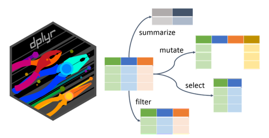
The term data manipulation might sound a bit tricky. However, it does not mean we plan to show you how to cheat and get better results. It simply means we want to show you how to easily handle the data and prepare it in the form you need. The functions for basic data handling, namely select(), filter(), mutate(), arrange(), and slice(), are provided by the tidyverse package dplyr. Do you remember how to find out more about the package? If nothing else, you can try ?dplyr, which actually gives you more hints where to look further.
Note that many of these operations can also be performed in some table editors (e.g., Excel) before importing to R. However, the effort and time demands would be significantly higher and would increase enormously with the size of the dataset. In contrast, in R, you can modify and rerun the steps in a single pipeline, and the data will be immediately ready for the following analysis.
We will need the following libraries:
And the forest understory dataset. Again, we will import the data just once and use the pipe to test the functions/effects without actually changing the data:
data <- read_excel("data/forest_understory/Axmanova-Forest-understory-diversity-analyses.xlsx")
names(data)
[1] "PlotID" "ForestType" "ForestTypeName" "Herbs"
[5] "Juveniles" "CoverE1" "Biomass" "Soil_depth_categ"
[9] "pH_KCl" "Slope" "Altitude" "Canopy_E3"
[13] "Radiation" "Heat" "TransDir" "TransDif"
[17] "TransTot" "EIV_light" "EIV_moisture" "EIV_soilreaction"
[21] "EIV_nutrients" "TWI" 2.2 select()
select() extracts columns/variables based on their names or position. It is essential to understand the distinction between select() and filter(). select() is used to select variables (columns) we want to keep in the dataset, while filter() applies to rows depending on their values.
You can select by naming the variables. Here, you would appreciate the tidy style of names! Tidy names mean no need to use parentheses :-).
data %>%
  select(PlotID, ForestType, ForestTypeName)
# A tibble: 65 × 3
PlotID ForestType ForestTypeName
<dbl> <dbl> <chr>
1 1 2 oak hornbeam forest
2 2 1 oak forest
3 3 1 oak forest
4 4 1 oak forest
5 5 1 oak forest
6 6 1 oak forest
7 7 1 oak forest
8 8 2 oak hornbeam forest
9 9 2 oak hornbeam forest
10 10 1 oak forest
# ℹ 55 more rowsYou can also select by position. However, be sure it will remain the same after all the changes you might make to the data.
data %>%
  select(1:3)
# A tibble: 65 × 3
PlotID ForestType ForestTypeName
<dbl> <dbl> <chr>
1 1 2 oak hornbeam forest
2 2 1 oak forest
3 3 1 oak forest
4 4 1 oak forest
5 5 1 oak forest
6 6 1 oak forest
7 7 1 oak forest
8 8 2 oak hornbeam forest
9 9 2 oak hornbeam forest
10 10 1 oak forest
# ℹ 55 more rowsSometimes, you decide you want to get rid of some variables. Either you can name all the others that you want to keep, or you can remove the unwanted ones with a minus sign. In the case of just one variable, it is easy: select(-xx). If you want to exclude two or more, you have to use select(-c(xx, xy)).
data %>%
  select(-c(ForestType, ForestTypeName))
# A tibble: 65 × 20
PlotID Herbs Juveniles CoverE1 Biomass Soil_depth_categ pH_KCl Slope Altitude
<dbl> <dbl> <dbl> <dbl> <dbl> <dbl> <dbl> <dbl> <dbl>
1 1 26 12 20 12.8 5 5.28 4 412
2 2 13 3 25 9.9 4.5 3.24 24 458
3 3 14 1 25 15.2 3 4.01 13 414
4 4 15 5 30 16 3 3.77 21 379
5 5 13 1 35 20.7 3 3.5 0 374
6 6 16 3 60 46.4 6 3.8 10 380
7 7 17 5 70 49.2 7 3.48 6 373
8 8 21 1 70 48.7 5 3.68 0 390
9 9 15 4 15 13.8 3.5 4.24 38 255
10 10 14 4 75 79.1 5 4.01 13 340
# ℹ 55 more rows
# ℹ 11 more variables: Canopy_E3 <dbl>, Radiation <dbl>, Heat <dbl>,
# TransDir <dbl>, TransDif <dbl>, TransTot <dbl>, EIV_light <dbl>,
# EIV_moisture <dbl>, EIV_soilreaction <dbl>, EIV_nutrients <dbl>, TWI <dbl>You can also define a range of variables between two of them.
data %>%
  select(PlotID:ForestTypeName)
# A tibble: 65 × 3
PlotID ForestType ForestTypeName
<dbl> <dbl> <chr>
1 1 2 oak hornbeam forest
2 2 1 oak forest
3 3 1 oak forest
4 4 1 oak forest
5 5 1 oak forest
6 6 1 oak forest
7 7 1 oak forest
8 8 2 oak hornbeam forest
9 9 2 oak hornbeam forest
10 10 1 oak forest
# ℹ 55 more rowsOr you can combine the approaches listed above:
data %>%
  select (PlotID, 3:6)
# A tibble: 65 × 5
PlotID ForestTypeName Herbs Juveniles CoverE1
<dbl> <chr> <dbl> <dbl> <dbl>
1 1 oak hornbeam forest 26 12 20
2 2 oak forest 13 3 25
3 3 oak forest 14 1 25
4 4 oak forest 15 5 30
5 5 oak forest 13 1 35
6 6 oak forest 16 3 60
7 7 oak forest 17 5 70
8 8 oak hornbeam forest 21 1 70
9 9 oak hornbeam forest 15 4 15
10 10 oak forest 14 4 75
# ℹ 55 more rowsselect() can also be used in combination with functions from the stringr package to identify a specific pattern in the names. Try several options: starts_with(), ends_with() or a more general one, contains().
data %>%
  select (PlotID, starts_with("EIV"))
# A tibble: 65 × 5
PlotID EIV_light EIV_moisture EIV_soilreaction EIV_nutrients
<dbl> <dbl> <dbl> <dbl> <dbl>
1 1 5 4.38 6.68 4.31
2 2 4.71 4.64 4.67 3.69
3 3 4.36 4.7 4.8 3.55
4 4 5.26 4.38 5.53 3.56
5 5 6.14 4 5.33 3.46
6 6 6.19 4.35 6.75 5.06
7 7 6.19 4.25 6.09 4.33
8 8 5.29 4.6 5.07 4.12
9 9 5.47 4.36 5.46 3.5
10 10 6.53 3.86 6 3
# ℹ 55 more rowsselect() can effectively help you organise the data. Imagine you have a workflow where you need only some variables, but in a specific sequence. And you import the data from different people or years. By using select() in your script, you can always order the variables in the same way, e.g., SampleID, ForestType, SpeciesNr, Productivity, even during import. You can also rename the variables using select to get exactly what you need. Here, the new name is on the left, as in rename().
data %>%
  select(SampleID = PlotID, ForestCode = ForestType, SpeciesNr = Herbs, Productivity = Biomass)
# A tibble: 65 × 4
SampleID ForestCode SpeciesNr Productivity
<dbl> <dbl> <dbl> <dbl>
1 1 2 26 12.8
2 2 1 13 9.9
3 3 1 14 15.2
4 4 1 15 16
5 5 1 13 20.7
6 6 1 16 46.4
7 7 1 17 49.2
8 8 2 21 48.7
9 9 2 15 13.8
10 10 1 14 79.1
# ℹ 55 more rows2.3 arrange()
This function retains the same variables and reorders the rows according to the values of the selected variables. To view the changes at a glance, we will first select only a few variables.
data <- read_excel("data/forest_understory/Axmanova-Forest-understory-diversity-analyses.xlsx")
data <- data %>% select(PlotID, ForestType, ForestTypeName, Biomass)
Now we have decided to arrange the data by Forest type.
data %>%
  arrange(ForestTypeName)
# A tibble: 65 × 4
PlotID ForestType ForestTypeName Biomass
<dbl> <dbl> <chr> <dbl>
1 101 4 alluvial forest 91.1
2 103 4 alluvial forest 114.
3 104 4 alluvial forest 188.
4 110 4 alluvial forest 126.
5 111 4 alluvial forest 84.8
6 113 4 alluvial forest 74.5
7 125 4 alluvial forest 123.
8 127 4 alluvial forest 176
9 129 4 alluvial forest 100.
10 131 4 alluvial forest 163.
# ℹ 55 more rowsWe can also decide to arrange the data from the highest value to the lowest, i.e. in descending order.
data %>%
  arrange(desc(Biomass))
# A tibble: 65 × 4
PlotID ForestType ForestTypeName Biomass
<dbl> <dbl> <chr> <dbl>
1 132 4 alluvial forest 287.
2 130 3 ravine forest 238
3 104 4 alluvial forest 188.
4 127 4 alluvial forest 176
5 131 4 alluvial forest 163.
6 110 4 alluvial forest 126.
7 125 4 alluvial forest 123.
8 128 3 ravine forest 121.
9 103 4 alluvial forest 114.
10 124 2 oak hornbeam forest 102.
# ℹ 55 more rowsOr we can arrange according to more variables. Here, the forest type is listed first, as we have decided it is the most important grouping variable. Within each type, we want to see the rows/cases ordered by biomass values.
data %>%
  arrange(ForestType, ForestTypeName, desc(Biomass)) %>% print(n = 30)
# A tibble: 65 × 4
PlotID ForestType ForestTypeName Biomass
<dbl> <dbl> <chr> <dbl>
1 10 1 oak forest 79.1
2 7 1 oak forest 49.2
3 6 1 oak forest 46.4
4 44 1 oak forest 34.1
5 82 1 oak forest 33.9
6 28 1 oak forest 29.7
7 42 1 oak forest 21.5
8 5 1 oak forest 20.7
9 81 1 oak forest 20.6
10 4 1 oak forest 16
11 47 1 oak forest 15.5
12 3 1 oak forest 15.2
13 31 1 oak forest 14.9
14 100 1 oak forest 13.5
15 2 1 oak forest 9.9
16 11 1 oak forest 7.4
17 124 2 oak hornbeam forest 102.
18 120 2 oak hornbeam forest 98.5
19 121 2 oak hornbeam forest 84.7
20 126 2 oak hornbeam forest 72.9
21 18 2 oak hornbeam forest 72.2
22 118 2 oak hornbeam forest 66.2
23 99 2 oak hornbeam forest 64.8
24 109 2 oak hornbeam forest 60.7
25 112 2 oak hornbeam forest 58.4
26 102 2 oak hornbeam forest 57.4
27 117 2 oak hornbeam forest 54.7
28 8 2 oak hornbeam forest 48.7
29 86 2 oak hornbeam forest 46.9
30 87 2 oak hornbeam forest 42.9
# ℹ 35 more rowsTo see more rows of the resulting table, we specified their number using the print() function.
2.4 distinct()
distinct() is a function that takes your data and removes all the duplicate rows, keeping only the unique ones. There are many cases where you will truly appreciate this elegant and effortless approach. For example, we want a list of unique Plot IDs, unique combinations of two categories, and so on. Here, we aim to compile a list of forest type codes and corresponding names.
data %>%
  arrange(ForestType) %>%
  select(ForestType, ForestTypeName) %>%
  distinct()
# A tibble: 4 × 2
ForestType ForestTypeName
<dbl> <chr>
1 1 oak forest
2 2 oak hornbeam forest
3 3 ravine forest
4 4 alluvial forest The same can also be done if I skip the select tool, because distinct() works more like select() + distinct().
data %>%
  arrange(ForestType) %>%
  distinct(ForestType, ForestTypeName)
# A tibble: 4 × 2
ForestType ForestTypeName
<dbl> <chr>
1 1 oak forest
2 2 oak hornbeam forest
3 3 ravine forest
4 4 alluvial forest Sometimes, distinct() can also be used when importing data to remove duplicate rows that were overlooked previously: data <- read_csv... %>% distinct().
2.5 filter() and slice()
When we have a large dataset, we sometimes need to create a subset of the rows/cases. First, we need to define the variable on which we will filter the rows (e.g., Forest type, soil pH) and determine which values are acceptable and which are not.
In this first example, we use a categorical variable, and we want to match the exact value, so we have to use ==
data %>%
  filter(ForestTypeName == "alluvial forest")
# A tibble: 11 × 4
PlotID ForestType ForestTypeName Biomass
<dbl> <dbl> <chr> <dbl>
1 101 4 alluvial forest 91.1
2 103 4 alluvial forest 114.
3 104 4 alluvial forest 188.
4 110 4 alluvial forest 126.
5 111 4 alluvial forest 84.8
6 113 4 alluvial forest 74.5
7 125 4 alluvial forest 123.
8 127 4 alluvial forest 176
9 129 4 alluvial forest 100.
10 131 4 alluvial forest 163.
11 132 4 alluvial forest 287. Or we might define a list of values, especially for categorical variables. The filter function will try to find rows with values exactly matching those %in% the list.
data %>%
  filter(ForestTypeName %in% c("alluvial forest", "ravine forest"))
# A tibble: 21 × 4
PlotID ForestType ForestTypeName Biomass
<dbl> <dbl> <chr> <dbl>
1 101 4 alluvial forest 91.1
2 103 4 alluvial forest 114.
3 104 4 alluvial forest 188.
4 105 3 ravine forest 65.5
5 106 3 ravine forest 33.6
6 108 3 ravine forest 82.3
7 110 4 alluvial forest 126.
8 111 4 alluvial forest 84.8
9 113 4 alluvial forest 74.5
10 114 3 ravine forest 71.5
# ℹ 11 more rowsWhen filtering a continuous variable, we can work with thresholds. For example, here the biomass of the herb layer is measured in g/m2, and we want only those rows/cases where the biomass values are higher than 80.
data <- read_excel("data/forest_understory/Axmanova-Forest-understory-diversity-analyses.xlsx")
data %>%
  filter(Biomass > 80) #[g/m2]
# A tibble: 17 × 22
PlotID ForestType ForestTypeName Herbs Juveniles CoverE1 Biomass
<dbl> <dbl> <chr> <dbl> <dbl> <dbl> <dbl>
1 101 4 alluvial forest 28 6 90 91.1
2 103 4 alluvial forest 35 5 80 114.
3 104 4 alluvial forest 25 11 85 188.
4 108 3 ravine forest 28 7 70 82.3
5 110 4 alluvial forest 37 4 95 126.
6 111 4 alluvial forest 26 10 85 84.8
7 120 2 oak hornbeam forest 36 6 75 98.5
8 121 2 oak hornbeam forest 30 12 80 84.7
9 122 3 ravine forest 29 6 60 102.
10 124 2 oak hornbeam forest 34 15 75 102.
11 125 4 alluvial forest 25 8 95 123.
12 127 4 alluvial forest 53 6 0 176
13 128 3 ravine forest 20 4 70 121.
14 129 4 alluvial forest 31 7 85 100.
15 130 3 ravine forest 18 5 85 238
16 131 4 alluvial forest 59 3 95 163.
17 132 4 alluvial forest 60 7 90 287.
# ℹ 15 more variables: Soil_depth_categ <dbl>, pH_KCl <dbl>, Slope <dbl>,
# Altitude <dbl>, Canopy_E3 <dbl>, Radiation <dbl>, Heat <dbl>,
# TransDir <dbl>, TransDif <dbl>, TransTot <dbl>, EIV_light <dbl>,
# EIV_moisture <dbl>, EIV_soilreaction <dbl>, EIV_nutrients <dbl>, TWI <dbl>You can also filter plots within a specified range and apply multiple conditions. Here, we want to keep only plots with biomass in the range of 40–80 g/m², but we also want to keep plots without a value (NA).
data %>%
  filter((Biomass >= 40 & Biomass <= 80) | is.na(Biomass))
# A tibble: 20 × 22
PlotID ForestType ForestTypeName Herbs Juveniles CoverE1 Biomass
<dbl> <dbl> <chr> <dbl> <dbl> <dbl> <dbl>
1 6 1 oak forest 16 3 60 46.4
2 7 1 oak forest 17 5 70 49.2
3 8 2 oak hornbeam forest 21 1 70 48.7
4 10 1 oak forest 14 4 75 79.1
5 18 2 oak hornbeam forest 13 3 85 72.2
6 86 2 oak hornbeam forest 32 5 40 46.9
7 87 2 oak hornbeam forest 34 9 65 42.9
8 99 2 oak hornbeam forest 18 6 85 64.8
9 102 2 oak hornbeam forest 37 13 65 57.4
10 105 3 ravine forest 12 10 80 65.5
11 109 2 oak hornbeam forest 25 9 50 60.7
12 112 2 oak hornbeam forest 32 14 60 58.4
13 113 4 alluvial forest 37 10 70 74.5
14 114 3 ravine forest 12 6 50 71.5
15 115 3 ravine forest 23 2 70 54.6
16 116 3 ravine forest 16 3 45 64.5
17 117 2 oak hornbeam forest 31 7 55 54.7
18 118 2 oak hornbeam forest 8 5 45 66.2
19 123 3 ravine forest 34 11 70 53.6
20 126 2 oak hornbeam forest 27 7 65 72.9
# ℹ 15 more variables: Soil_depth_categ <dbl>, pH_KCl <dbl>, Slope <dbl>,
# Altitude <dbl>, Canopy_E3 <dbl>, Radiation <dbl>, Heat <dbl>,
# TransDir <dbl>, TransDif <dbl>, TransTot <dbl>, EIV_light <dbl>,
# EIV_moisture <dbl>, EIV_soilreaction <dbl>, EIV_nutrients <dbl>, TWI <dbl>Example of multiple conditions in one filter line. Here, we select all plots of the specified types and exclude the others, taking only those with higher biomass, because we used the OR (|) operator between the two conditions.
data %>%
  filter((ForestTypeName %in% c("alluvial forest", "ravine forest") |
    (Biomass >= 80)))
# A tibble: 24 × 22
PlotID ForestType ForestTypeName Herbs Juveniles CoverE1 Biomass
<dbl> <dbl> <chr> <dbl> <dbl> <dbl> <dbl>
1 101 4 alluvial forest 28 6 90 91.1
2 103 4 alluvial forest 35 5 80 114.
3 104 4 alluvial forest 25 11 85 188.
4 105 3 ravine forest 12 10 80 65.5
5 106 3 ravine forest 16 0 75 33.6
6 108 3 ravine forest 28 7 70 82.3
7 110 4 alluvial forest 37 4 95 126.
8 111 4 alluvial forest 26 10 85 84.8
9 113 4 alluvial forest 37 10 70 74.5
10 114 3 ravine forest 12 6 50 71.5
# ℹ 14 more rows
# ℹ 15 more variables: Soil_depth_categ <dbl>, pH_KCl <dbl>, Slope <dbl>,
# Altitude <dbl>, Canopy_E3 <dbl>, Radiation <dbl>, Heat <dbl>,
# TransDir <dbl>, TransDif <dbl>, TransTot <dbl>, EIV_light <dbl>,
# EIV_moisture <dbl>, EIV_soilreaction <dbl>, EIV_nutrients <dbl>, TWI <dbl>Sometimes you might find it useful to filter something out, rather than specifying what should stay. This is indicated by the exclamation mark, as shown below.
data %>%
  filter(!is.na(Juveniles))
# A tibble: 65 × 22
PlotID ForestType ForestTypeName Herbs Juveniles CoverE1 Biomass
<dbl> <dbl> <chr> <dbl> <dbl> <dbl> <dbl>
1 1 2 oak hornbeam forest 26 12 20 12.8
2 2 1 oak forest 13 3 25 9.9
3 3 1 oak forest 14 1 25 15.2
4 4 1 oak forest 15 5 30 16
5 5 1 oak forest 13 1 35 20.7
6 6 1 oak forest 16 3 60 46.4
7 7 1 oak forest 17 5 70 49.2
8 8 2 oak hornbeam forest 21 1 70 48.7
9 9 2 oak hornbeam forest 15 4 15 13.8
10 10 1 oak forest 14 4 75 79.1
# ℹ 55 more rows
# ℹ 15 more variables: Soil_depth_categ <dbl>, pH_KCl <dbl>, Slope <dbl>,
# Altitude <dbl>, Canopy_E3 <dbl>, Radiation <dbl>, Heat <dbl>,
# TransDir <dbl>, TransDif <dbl>, TransTot <dbl>, EIV_light <dbl>,
# EIV_moisture <dbl>, EIV_soilreaction <dbl>, EIV_nutrients <dbl>, TWI <dbl>A specific alternative to filter() is the slice() function. Let’s say I want to get the top 3 rows/cases/vegetation samples with the highest numbers of recorded juveniles. So, we can arrange the values, determine the threshold and filter the values above it. Or we can use slice_max() to do the job for us.
data %>%
  filter(!is.na(Juveniles)) %>%
  slice_max(Juveniles, n = 3)
# A tibble: 3 × 22
PlotID ForestType ForestTypeName Herbs Juveniles CoverE1 Biomass
<dbl> <dbl> <chr> <dbl> <dbl> <dbl> <dbl>
1 124 2 oak hornbeam forest 34 15 75 102.
2 112 2 oak hornbeam forest 32 14 60 58.4
3 119 2 oak hornbeam forest 63 14 50 36.6
# ℹ 15 more variables: Soil_depth_categ <dbl>, pH_KCl <dbl>, Slope <dbl>,
# Altitude <dbl>, Canopy_E3 <dbl>, Radiation <dbl>, Heat <dbl>,
# TransDir <dbl>, TransDif <dbl>, TransTot <dbl>, EIV_light <dbl>,
# EIV_moisture <dbl>, EIV_soilreaction <dbl>, EIV_nutrients <dbl>, TWI <dbl>Tip: Try slice_min() if you need the lowest values.
2.6 mutate()
mutate() adds new variables that are functions of existing variables, e.g. round the values. It can also overwrite the original variable.
For example, in the field, I recorded juveniles of woody plants and all other herb-layer species separately. However, we now want to sum these two values for each row/case/vegetation plot so that we can speak about overall species richness. I create a new variable by simply summing these two (note how easy it is with tidy names!).
data %>%
  mutate(SpeciesRichness = Herbs + Juveniles) %>%
  select(PlotID, SpeciesRichness, Herbs, Juveniles)
# A tibble: 65 × 4
PlotID SpeciesRichness Herbs Juveniles
<dbl> <dbl> <dbl> <dbl>
1 1 38 26 12
2 2 16 13 3
3 3 15 14 1
4 4 20 15 5
5 5 14 13 1
6 6 19 16 3
7 7 22 17 5
8 8 22 21 1
9 9 19 15 4
10 10 18 14 4
# ℹ 55 more rowsSometimes, you want to add a variable where all rows/cases will receive the same value. For example, because you plan to join the data with other data or because it is useful for another mutate(). This is also a straightforward method for converting data with abundances to presence/absence data.
data %>%
  mutate(selection = 1)%>%
  select(PlotID, selection, ForestType, ForestTypeName)
# A tibble: 65 × 4
PlotID selection ForestType ForestTypeName
<dbl> <dbl> <dbl> <chr>
1 1 1 2 oak hornbeam forest
2 2 1 1 oak forest
3 3 1 1 oak forest
4 4 1 1 oak forest
5 5 1 1 oak forest
6 6 1 1 oak forest
7 7 1 1 oak forest
8 8 1 2 oak hornbeam forest
9 9 1 2 oak hornbeam forest
10 10 1 1 oak forest
# ℹ 55 more rowsYou can also create a variable with more categories based on the values of other variables using ifelse() inside mutate(). You give the condition when it should be called ‘low’ and what to do if the condition is not met - name it ‘high’.
Tip: Inside ‘Condition’, you can also use other conditional operators, like AND (&), OR (|), or EQUAL (==).
data %>%
  mutate(Productivity = ifelse(Biomass<60,"low","high")) %>%
  select (PlotID, ForestTypeName, Productivity, Biomass) %>%
  print(n=20)
# A tibble: 65 × 4
PlotID ForestTypeName Productivity Biomass
<dbl> <chr> <chr> <dbl>
1 1 oak hornbeam forest low 12.8
2 2 oak forest low 9.9
3 3 oak forest low 15.2
4 4 oak forest low 16
5 5 oak forest low 20.7
6 6 oak forest low 46.4
7 7 oak forest low 49.2
8 8 oak hornbeam forest low 48.7
9 9 oak hornbeam forest low 13.8
10 10 oak forest high 79.1
11 11 oak forest low 7.4
12 14 oak hornbeam forest low 14.2
13 16 oak hornbeam forest low 26.2
14 18 oak hornbeam forest high 72.2
15 28 oak forest low 29.7
16 29 oak hornbeam forest low 37.9
17 31 oak forest low 14.9
18 32 oak hornbeam forest low 19.2
19 36 oak hornbeam forest low 3.3
20 41 oak hornbeam forest low 26.9
# ℹ 45 more rowsThe same can be done with a similar approach using case_when(). Conditions are evaluated from the first (on the left) to the last (on the right side), so for each step, you take only the rows that are not yet treated by the previous condition.
data %>%
  mutate(Productivity = case_when(Biomass <= 60 ~ "low", Biomass > 60 ~ "high")) %>%
  select(PlotID, ForestTypeName, Productivity, Biomass) %>%
  print(n = 20)
# A tibble: 65 × 4
PlotID ForestTypeName Productivity Biomass
<dbl> <chr> <chr> <dbl>
1 1 oak hornbeam forest low 12.8
2 2 oak forest low 9.9
3 3 oak forest low 15.2
4 4 oak forest low 16
5 5 oak forest low 20.7
6 6 oak forest low 46.4
7 7 oak forest low 49.2
8 8 oak hornbeam forest low 48.7
9 9 oak hornbeam forest low 13.8
10 10 oak forest high 79.1
11 11 oak forest low 7.4
12 14 oak hornbeam forest low 14.2
13 16 oak hornbeam forest low 26.2
14 18 oak hornbeam forest high 72.2
15 28 oak forest low 29.7
16 29 oak hornbeam forest low 37.9
17 31 oak forest low 14.9
18 32 oak hornbeam forest low 19.2
19 36 oak hornbeam forest low 3.3
20 41 oak hornbeam forest low 26.9
# ℹ 45 more rowsI have already said that we often use mutate() to transform original values directly. To work with multiple variables at once, e.g., round them, we can use mutate(across()).
data %>%
  mutate(across(c(Biomass, pH_KCl, TransTot), ~ round(.x, digits = 1))) %>%
  select(PlotID, Biomass, pH_KCl, TransTot)
# A tibble: 65 × 4
PlotID Biomass pH_KCl TransTot
<dbl> <dbl> <dbl> <dbl>
1 1 12.8 5.3 6.6
2 2 9.9 3.2 6.9
3 3 15.2 4 7.3
4 4 16 3.8 6.4
5 5 20.7 3.5 6.9
6 6 46.4 3.8 7
7 7 49.2 3.5 7.4
8 8 48.7 3.7 7
9 9 13.8 4.2 6.5
10 10 79.1 4 6.3
# ℹ 55 more rows.x refers to the entire column (vector) being transformed inside a function like mutate(across(...)) or map().
2.7 Save the data
If you decide that you have already prepared the dataset in the form it should be used later, you probably need to save it and export, e.g. as a csv. Remember that we were primarily trying to see what it would look like with the %>%, so you must either assign the dataset to a new name or add the write command at the end of the pipeline. See also Chapter 1.
Here we will play a bit with the tidyverse package readr.
Write a comma-delimited file:
write_csv(data, "exercisesIA/forest_selected1.csv") Write a semicolon-delimited file (;):
write_csv2(data, "exercisesIA/forest_selected2.csv")Or find out more in the readr cheatsheet. Note that, in contrast to the write.csv() function, the write_csv() function adheres to the tidyverse philosophy, so row names are not included in the export.
You can also write directly to an Excel file, for example, using the writexl library.
library(writexl)
write_xlsx(data, 'exercisesIA/forestEnv.xlsx')
To create an xlsx with (multiple) named sheets, you would need to provide a list of data frames. Here, we specify that data1 should be saved as an Excel sheet named forestEnv (environmental data) and data2 as a sheet named forestSpe (species data from the same dataset).
library(writexl)
data1 <- read_excel("data/forest_understory/Axmanova-Forest-understory-diversity-analyses.xlsx")
data2 <- read_excel("data/forest_understory/Axmanova-Forest-spe.xlsx")
write_xlsx(list(forestEnv = data1, forestSpe = data2), 'exercisesIA/forest.xlsx' )
2.8 Exercises
1. Forest Data - Axmanova-Forest-understory-diversity-analyses.xlsx - download the data from the repository and save it into your project folder (Link to Github folder). This dataset is used throughout the whole chapter. Please use it to prepare your own script with remarks, copy and train what is described above.
Tip: If you copy the description and add it directly to your script, it is simply too long, right? Do you know how to read long lines of text in an R script? Go to “Code” and tick “soft wrap long lines”.
2. Directly from R Studio, create a folder results/chapter2 for saving today’s datasets, as we will train a bit of exporting the data.
3. Use the Forest Data to train more. Create variable “author” which will contain the name Axmanova > as we did before, create variable richness summing the herbs and juveniles > select variables plotID, author, richness, productivity (renamed biomass) and pH. Try to save this subset into results/chapter2.
4. Use the Forest dataset again. Find five plots with the lowest biomass from forest types other than oak forests.
5. Select PlotID and all variables that are connected to transmitted light (Trans..) > round these variables.
6. We will switch to another dataset, Species Forest Data - Axmanova-Forest-spe.xlsx - download the data from the repository and save it into your project folder (Link to Github folder). This is a long-format of the plant species recorded in the vegetation plots. Long format means that the records of species from one site are grouped by the same ID (here as RELEVE_NR). For each species, it is indicated in which vegetation layer it occurred, and an estimation of its abundance is in the form of percentage cover.
Import the data and check the structure > change it to presence-absence data (abundance set to 1) *Alternatively, prepare presence-absence data without considering different layers and save both lists on two different sheets of the Excel file.
7. Stay with the same dataset, we will try to get the list of all species occurring in the tree layer. Import the data > sort the species data alphabetically > get the list of unique species names of the tree layer (i.e. layer == 1) > print, view all the species or store them as a new dataset. Save the result into csv file.
8. iris dataset: We will use the famous iris dataset of flower measurements. Find out more details by asking R ?iris as the dataset is integrated and ready to use. Check the structure of the dataset > select variables including species and those of length measurements > arrange according to Sepal.Length > and filter 15 rows with the longest sepals. Which species prevails among these top 15?
9. squirrel data: Load data of squirrel observations from the Central Park Squirrel Census using this line: read_csv(‘https://raw.githubusercontent.com/rfordatascience/tidytuesday/main/data/2023/2023-05-23/squirrel_data.csv’)
Load squirrels data, check the structure, rename variables to get tidy names > find out what are the possible colours of fur > select at least 5 variables, including ID, fur colour, location, … > filter squirrels of one fur colour, up to your preference > arrange data by location > print at least 30 rows
- *get back to Forest data and using
case_when()define three levels of productivity: low, medium, and high.
2.9 Further reading
dplyr main web page: https://dplyr.tidyverse.org
Find dplyr Cheatsheet in Posit: https://posit.co/resources/cheatsheets/
Chapter devoted to Data transformation in the R for Data Science book: https://r4ds.hadley.nz/data-transform.html
encoding issues during import and export: https://irene.rbind.io/post/encoding-in-r/