library(tidyverse)1 Introduction
In this chapter, we will learn how to prepare for analyses in R, including preparing the project, starting a script, importing data, and conducting an initial exploration. We will follow the rules for preparing reproducible, reportable, clean and tidy workflow and scripts.
You already know that R is a programming language and environment for statistical analysis and data visualisation. R is a free and open-source software, available from the CRAN directory. R is extended by a large number of software packages, which contain reusable code, documentation, and sample data. In this course, we will focus primarily on the tidyverse collection of packages, which are designed for everyday data handling and visualisation (see more here).
We will work with R using the interface called RStudio IDE, in short RStudio, which is an integrated development environment for R and can be downloaded here.
TO DO: install R, RStudio and tidyverse package. Having trouble and need advice? Try the further reading section at the end of this chapter, or come and ask before the first lesson.
1.1. Introducing Tidyverse
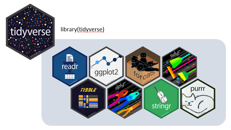
tidyverse is a collection of R packages for transforming and visualising data, which share an underlying philosophy (tidy data, tibbles, %>%) and a common interface. When you install the tidyverse, you get all the core packages at once, namely
readrfor data importingdplyrwith tools for data manipulation (e.g.select(),filter(),arrange(),mutate()…)tidyrwith functions that help you get to tidy data and transform their format (e.g.pivot)tibbleintroducing simple data frames called tibblesggplot2package for data visualisationstringrfor working with strings, matching defined patterns, and cleaning unwanted partsforcats, which enables easier work with factorslubridatehelps to work with dates and timespurrr, which offers a complete and consistent set of tools for working with functions and vectors, introducesmapfunctions instead of complicated loops
In addition, you get automatically installed several more packages, which share the same approach, although developed later or by someone else, for example, readxl, for elegant direct import from Excel files, or magrittr package, where the pipe was initially introduced, including double-sided pipe
Find more about tidyverse here or check cheatsheets and vignettes for individual packages.
Remember that all the core packages are activated within the tidyverse library,
while for the extra ones, you have to use an extra call:
library(readxl)1.1.1 Tidy data
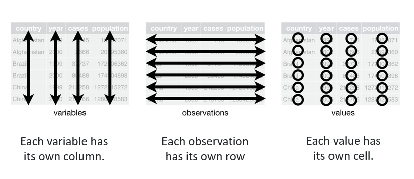
Data that are easy to handle and analyse.
Find more in the R for data science book: https://r4ds.hadley.nz/
1.1.2 Tibbles
Tibbles are new, updated versions of base-R data frames. They are designed to work better with other tidyverse packages. In contrast to data frames, tibbles never convert the type of the inputs (e.g. strings to factors), they never change the names of variables, and they never create row names. Example:
data <- read_excel("data/forest_understory/Axmanova-Forest-understory-diversity-analyses.xlsx")
tibble(data)
# A tibble: 65 × 22
PlotID ForestType ForestTypeName Herbs Juveniles CoverE1 Biomass
<dbl> <dbl> <chr> <dbl> <dbl> <dbl> <dbl>
1 1 2 oak hornbeam forest 26 12 20 12.8
2 2 1 oak forest 13 3 25 9.9
3 3 1 oak forest 14 1 25 15.2
4 4 1 oak forest 15 5 30 16
5 5 1 oak forest 13 1 35 20.7
6 6 1 oak forest 16 3 60 46.4
7 7 1 oak forest 17 5 70 49.2
8 8 2 oak hornbeam forest 21 1 70 48.7
9 9 2 oak hornbeam forest 15 4 15 13.8
10 10 1 oak forest 14 4 75 79.1
# ℹ 55 more rows
# ℹ 15 more variables: Soil_depth_categ <dbl>, pH_KCl <dbl>, Slope <dbl>,
# Altitude <dbl>, Canopy_E3 <dbl>, Radiation <dbl>, Heat <dbl>,
# TransDir <dbl>, TransDif <dbl>, TransTot <dbl>, EIV_light <dbl>,
# EIV_moisture <dbl>, EIV_soilreaction <dbl>, EIV_nutrients <dbl>, TWI <dbl>1.1.3 Pipes %>%
The tidyverse tools use a pipe: %>% or |>. The pipe allows the output of a previous command to be used as input to another command, rather than using nested functions. It means that a pipe binds individual steps into a sequence, and it reads from left to right. In base R, the logic of reading is from inside out, and you have to save all the steps separately.
See this example of the same steps with different approaches:
Base R method:
data <- read_excel("data/forest_understory/Axmanova-Forest-understory-diversity-analyses.xlsx")
# 1. Create a new variable in the data
data$Productivity <- ifelse(data$Biomass < 60, "low", "high")

# 2. Select only some columns, save as a new dataframe
df <- data[, c("PlotID", "ForestTypeName", "Productivity", "pH_KCl")]

# 3. Order by soil pH (descending)
df <- df[order(df$pH_KCl, decreasing = TRUE), ]

# 4. Keep only the first 15 rows with the highest pH
df_top15 <- df[1:15, ]

# 5. Print the resulting subset to see which forest types grow in the high pH soils and if they have rather low or high productivity
df_top15
# A tibble: 15 × 4
PlotID ForestTypeName Productivity pH_KCl
<dbl> <chr> <chr> <dbl>
1 104 alluvial forest high 7.14
2 103 alluvial forest high 7.13
3 128 ravine forest high 7.03
4 111 alluvial forest high 7.01
5 114 ravine forest high 6.93
6 123 ravine forest low 6.91
7 105 ravine forest high 6.78
8 122 ravine forest high 6.68
9 101 alluvial forest high 6.67
10 119 oak hornbeam forest low 6.63
11 113 alluvial forest high 6.61
12 120 oak hornbeam forest high 6.42
13 115 ravine forest low 6.03
14 110 alluvial forest high 5.82
15 121 oak hornbeam forest high 5.77Piping (the same steps, but just in one line):
data <- read_excel("data/forest_understory/Axmanova-Forest-understory-diversity-analyses.xlsx") %>%
  mutate(Productivity = ifelse(Biomass < 100, "low", "high")) %>%
  select(PlotID, ForestTypeName, Productivity, pH_KCl) %>%
  arrange(desc(pH_KCl)) %>%
  slice_head(n = 15) %>%
  print()
# A tibble: 15 × 4
PlotID ForestTypeName Productivity pH_KCl
<dbl> <chr> <chr> <dbl>
1 104 alluvial forest high 7.14
2 103 alluvial forest high 7.13
3 128 ravine forest high 7.03
4 111 alluvial forest low 7.01
5 114 ravine forest low 6.93
6 123 ravine forest low 6.91
7 105 ravine forest low 6.78
8 122 ravine forest high 6.68
9 101 alluvial forest low 6.67
10 119 oak hornbeam forest low 6.63
11 113 alluvial forest low 6.61
12 120 oak hornbeam forest low 6.42
13 115 ravine forest low 6.03
14 110 alluvial forest high 5.82
15 121 oak hornbeam forest low 5.77Note: It is even possible to overwrite the original dataset with an assignment pipe %<>% included in the magrittr package. We will try to avoid this in our lessons, as it cannot be undone.
Tip: Insert a pipe by Ctrl + Shift + M.
1.2. Effective and reproducible workflow
There are several rules to make your workflow effective and reproducible after some time or by other people.
1.2.1 Projects
If you start your work by setting the working directory, the reproducibility by someone else is very limited (see more here). A good habit is to organise each data analysis into a project: a folder on your computer that holds all the files relevant to that particular piece of work.
R Studio easily enables creating projects and switching between them (either through File > Open/New/Recent Project or by clicking the upper-right corner icon for projects).
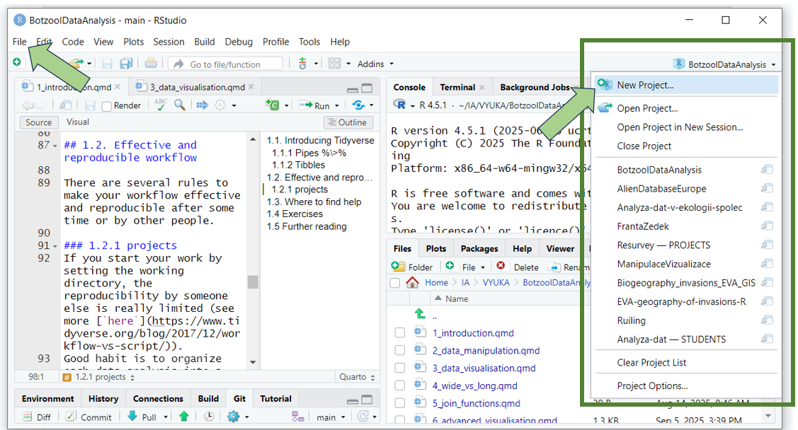
Tip: get used to creating the same subfolders in each of your projects: data, scripts, results, maps, backup, etc., to further organise the project structure. If you save the data into them, you can directly import them and view them through the project in R Studio.
1.2.2 Scripts
- libraries
- list all the libraries your code needs at the beginning of the script
library(tidyverse)
library(readxl)- remarks
- add notes to your scripts, you will be grateful later
- change the text to non-active (marked with hash tags
#)Ctrl + Shift + C
- separate scripts or sections
- insert named section using
Ctrl + Shift + R - or divide the code by
#### - fold all sections with
Alt + O - unfold all with
Shift + Alt + O
- insert named section using
- variable names
- should be short and easy to handle, without spaces, strange symbols
- Simple variable names will save you a great deal of time and effort, as well as the need for parentheses.
See this example:
data <- read_csv("data/messy_data/Example0.csv")
names(data)
[1] "Relevé number" "Taxon"
[3] "Vegetation layer" "Cover %"
[5] "Braun-Blanquet Scale (New) Code"You can rename strange names one by one. First, use the new name and place the old one on the right, as shown in the example below.
data %>% rename(Releve = "Relevé number")# A tibble: 51 × 5
Releve Taxon `Vegetation layer` `Cover %` Braun-Blanquet Scale…¹
<dbl> <chr> <dbl> <dbl> <chr>
1 435469 Ribes uva-crispa 0 2 +
2 435469 Ulmus minor 0 3 1
3 435469 Crataegus monogyn… 0 2 +
4 435469 Rubus caesius 0 13 a
5 435469 Prunus padus ssp.… 0 3 1
6 435469 Populus alba 0 13 a
7 435469 Fraxinus excelsior 0 68 4
8 435469 Arctium lappa 6 1 r
9 435469 Adoxa moschatelli… 6 2 +
10 435469 Aegopodium podagr… 6 13 a
# ℹ 41 more rows
# ℹ abbreviated name: ¹`Braun-Blanquet Scale (New) Code`Alternatively, you can change all complex patterns at once, using RegEx regular expressions. Import the example once again.
You identify the pattern on the left, starting with two backslashes and define the outcome on the right side. Be sure to keep the logic in your sequence - what is first and what last, as it really changes the patterns one by one, as they are listed.
data <- read_csv("data/messy_data/Example0.csv")
names(data)
[1] "Relevé number" "Taxon"
[3] "Vegetation layer" "Cover %"
[5] "Braun-Blanquet Scale (New) Code"data %>%
rename_all(~ str_replace_all(., c(
"\\." = "", # remove dots in the variable names
"\\é" = "e", # replace é by e
"\\%" = "perc", # remove symbol % and change it to perc
"\\(" = "", # remove brackets
"\\)" = "", # remove brackets
"\\/" = "", # remove slash
"\\?" = "", # remove questionmark
"\\s" = "."))) # remove spaces# A tibble: 51 × 5
Releve.number Taxon Vegetation.layer Cover.perc Braun-Blanquet.Scale…¹
<dbl> <chr> <dbl> <dbl> <chr>
1 435469 Ribes uva-c… 0 2 +
2 435469 Ulmus minor 0 3 1
3 435469 Crataegus m… 0 2 +
4 435469 Rubus caesi… 0 13 a
5 435469 Prunus padu… 0 3 1
6 435469 Populus alba 0 13 a
7 435469 Fraxinus ex… 0 68 4
8 435469 Arctium lap… 6 1 r
9 435469 Adoxa mosch… 6 2 +
10 435469 Aegopodium … 6 13 a
# ℹ 41 more rows
# ℹ abbreviated name: ¹`Braun-Blanquet.Scale.New.Code`Now check the names again. Did it work?
- Tip: Use the function
clean_names()from thejanitorpackage
Note that in the examples above, you are not really rewriting the data you have imported. Here, the data %>% means that you are just trying to see what it would look like if you apply the following steps to the data. To really change it, you would have to assign your result to a new dataset by using one of the following options:
data2 <- data1 %>%… # defining first the new datasetdata <- data %>%… # rewriting the existing datasetdata %<>% data… # rewriting the existing dataset by assignment pipe (magrittr)data1 %>% ...-> data2# making/testing all the steps and assigning it to a new dataset as the last step
This might sound troublesome, but it is actually very helpful. You can try all the steps, and when you are satisfied with the code, you can combine everything into a single pipeline, from importing the data to exporting the result.
1.3 Data import
We will train on how to import data using the tidyverse approach, which includes readr or readxl for Excel files (see the cheatsheet).
It is useful to check which files are stored in the folders we have. Here, we list all files in the working (=project) directory.
list.files() [1] "1_introduction.qmd" "1_introduction.rmarkdown"
[3] "11_database_to_plot.html" "11_database_to_plot.qmd"
[5] "11_database_to_plot_files" "12_github.html"
[7] "12_github.qmd" "2_data_manipulation.qmd"
[9] "3_data_visualisation.qmd" "4_wide_vs_long.qmd"
[11] "5_join_functions.qmd" "6_advanced_visualisation.qmd"
[13] "7_8_automatisation.qmd" "9_10_maps.qmd"
[15] "apa.csl" "data"
[17] "data_manipulation_visualisation.qmd" "exercises"
[19] "images" "maps"
[21] "plots" "references.bib"
[23] "results" "scripts" Or we can dive deeper into the hierarchy and check the content of the data folder or a specific subfolder.
list.files("data") [1] "acidophilous_grasslands" "basiphilous_grasslands"
[3] "climate_raster" "dem_JMK"
[5] "forest_understory" "frogs"
[7] "frogs_territory" "frozen_fauna"
[9] "gapminder" "gapminder_clean"
[11] "gapminder_continent" "grasslands_shp"
[13] "lepidoptera" "messy_data"
[15] "Pladias_data" "regions"
[17] "sands" "soil_pH_LUCAS"
[19] "spruce_forest_wide_long" "turboveg_to_R"
[21] "vegetation_plots_JMK" list.files("data/forest_understory")[1] "Axmanova-Forest-env.xlsx"
[2] "Axmanova-Forest-spe.xlsx"
[3] "Axmanova-Forest-understory-diversity-analyses.xlsx"
[4] "Axmanova-Forest-understory-diversity-merged-long.xlsx"
[5] "readme.txt"
[6] "traits.xlsx" Let’s select one of the files and import it into our working environment. Depending on the type of file, we must select the appropriate approach. Here it is an Excel file, so I can use the read_excel() function. Check the cheatsheet for more tips.
data <- read_excel("data/forest_understory/Axmanova-Forest-understory-diversity-analyses.xlsx")We imported the data, and here are a few tips on how to check the structure.
First is the tibble, which appears automatically after any import using the tidyverse approach. Note that only ten rows and several variables are shown. If there are too many, the remaining variables are listed below.
tibble(data)# A tibble: 65 × 22
PlotID ForestType ForestTypeName Herbs Juveniles CoverE1 Biomass
<dbl> <dbl> <chr> <dbl> <dbl> <dbl> <dbl>
1 1 2 oak hornbeam forest 26 12 20 12.8
2 2 1 oak forest 13 3 25 9.9
3 3 1 oak forest 14 1 25 15.2
4 4 1 oak forest 15 5 30 16
5 5 1 oak forest 13 1 35 20.7
6 6 1 oak forest 16 3 60 46.4
7 7 1 oak forest 17 5 70 49.2
8 8 2 oak hornbeam forest 21 1 70 48.7
9 9 2 oak hornbeam forest 15 4 15 13.8
10 10 1 oak forest 14 4 75 79.1
# ℹ 55 more rows
# ℹ 15 more variables: Soil_depth_categ <dbl>, pH_KCl <dbl>, Slope <dbl>,
# Altitude <dbl>, Canopy_E3 <dbl>, Radiation <dbl>, Heat <dbl>,
# TransDir <dbl>, TransDif <dbl>, TransTot <dbl>, EIV_light <dbl>,
# EIV_moisture <dbl>, EIV_soilreaction <dbl>, EIV_nutrients <dbl>, TWI <dbl>An alternative way is to use glimpse(), where the variables are listed below each other, showing the first 15 values:
glimpse(data)Rows: 65
Columns: 22
$ PlotID <dbl> 1, 2, 3, 4, 5, 6, 7, 8, 9, 10, 11, 14, 16, 18, 28, 29…
$ ForestType <dbl> 2, 1, 1, 1, 1, 1, 1, 2, 2, 1, 1, 2, 2, 2, 1, 2, 1, 2,…
$ ForestTypeName <chr> "oak hornbeam forest", "oak forest", "oak forest", "o…
$ Herbs <dbl> 26, 13, 14, 15, 13, 16, 17, 21, 15, 14, 12, 30, 24, 1…
$ Juveniles <dbl> 12, 3, 1, 5, 1, 3, 5, 1, 4, 4, 4, 3, 7, 3, 1, 2, 2, 7…
$ CoverE1 <dbl> 20, 25, 25, 30, 35, 60, 70, 70, 15, 75, 8, 30, 60, 85…
$ Biomass <dbl> 12.8, 9.9, 15.2, 16.0, 20.7, 46.4, 49.2, 48.7, 13.8, …
$ Soil_depth_categ <dbl> 5.0, 4.5, 3.0, 3.0, 3.0, 6.0, 7.0, 5.0, 3.5, 5.0, 2.0…
$ pH_KCl <dbl> 5.28, 3.24, 4.01, 3.77, 3.50, 3.80, 3.48, 3.68, 4.24,…
$ Slope <dbl> 4, 24, 13, 21, 0, 10, 6, 0, 38, 13, 29, 47, 33, 24, 0…
$ Altitude <dbl> 412, 458, 414, 379, 374, 380, 373, 390, 255, 340, 368…
$ Canopy_E3 <dbl> 80, 80, 80, 75, 70, 65, 65, 85, 80, 70, 85, 60, 75, 7…
$ Radiation <dbl> 0.8813, 0.9329, 0.9161, 0.9305, 0.8691, 0.9178, 0.829…
$ Heat <dbl> 0.8575, 0.8138, 0.8503, 0.9477, 0.8691, 0.8834, 0.803…
$ TransDir <dbl> 3.72, 4.05, 4.38, 3.48, 3.73, 3.59, 4.49, 3.97, 3.61,…
$ TransDif <dbl> 2.83, 2.83, 2.94, 2.96, 3.15, 3.40, 2.87, 2.99, 2.92,…
$ TransTot <dbl> 6.55, 6.88, 7.31, 6.44, 6.88, 6.99, 7.36, 6.96, 6.53,…
$ EIV_light <dbl> 5.00, 4.71, 4.36, 5.26, 6.14, 6.19, 6.19, 5.29, 5.47,…
$ EIV_moisture <dbl> 4.38, 4.64, 4.70, 4.38, 4.00, 4.35, 4.25, 4.60, 4.36,…
$ EIV_soilreaction <dbl> 6.68, 4.67, 4.80, 5.53, 5.33, 6.75, 6.09, 5.07, 5.46,…
$ EIV_nutrients <dbl> 4.31, 3.69, 3.55, 3.56, 3.46, 5.06, 4.33, 4.12, 3.50,…
$ TWI <dbl> 3.353962, 2.419177, 2.159580, 1.651170, 4.741780, 2.4…If you forget the names of variables or you want to copy them and store them in your script, simply use names():
names(data) [1] "PlotID" "ForestType" "ForestTypeName" "Herbs"
[5] "Juveniles" "CoverE1" "Biomass" "Soil_depth_categ"
[9] "pH_KCl" "Slope" "Altitude" "Canopy_E3"
[13] "Radiation" "Heat" "TransDir" "TransDif"
[17] "TransTot" "EIV_light" "EIV_moisture" "EIV_soilreaction"
[21] "EIV_nutrients" "TWI" A quite useful base R function is table(), which shows the counts per category of the selected variable. In the tidyverse, it will require more steps to be completed, but we will get there next time.
table(data$ForestTypeName)
    alluvial forest          oak forest oak hornbeam forest       ravine forest
                 11                  16                  28                  10
Of course, you can also view() the data or click on it in the list in the Files pane to open it in a table-like scrollable format, which can be useful many times. However, this is not recommended for huge tables, as the previews are rather memory-intensive.
1.4 Where to find help
Motto: The majority of the problems in R can be solved if you know how to ask and where.
Knowing that I am lost in “Regular expressions” already helps me to ask more specifically.
R Studio help - Try the integrated help in R Studio, where you can find links to selected manuals and cheatsheets. It is also the place where you can find keyboard shortcut help to find out which combinations do what. e.g.
Ctrl + Shift + mCheatsheets - the most important features of a given package summarised on two A4 pages, ready to print
Vignettes are supporting documents that are available for many packages. They give examples and explain functions available in the package. You can discover vignettes by accessing the help page for a package, or via the
browseVignettes()function, which will get you to the overall list. Or you can try by typing specific names, e.g.,vignette("dplyr")R Studio community - Questions are sorted by packages, making it nice to check when looking for frequently asked questions.
Stack Overflow - You probably already came across Stack Overflow when you were trying to Google something, as it suggests answers to coding-related questions. It is a good environment to ask questions or try to find out if somebody has already asked the same things before. Be specific about the coding style. E.g. How to separate a variable using tidyverse?
GitHub is a great source - you can find data, projects, packages, and instructions there. If you stay till the end of this course, we will show you more.
AI tools are worth asking. For example (i), you have a code and you do not understand it, so you can ask for explanation, or (ii) you want to get the code translated to another syntax (e.g. from base R to tidyverse), (iii) or you want to know how to code something but you do not have a clue which packages to use… We will train this a bit.
Or just come and ask!
1.5 Exercises
For exercises, we will use either data that are published somewhere and give you the link, or we will ask you to download the data from the repository and save it into your project folder: Link to Github folder
There will be some obligatory tasks, while voluntary tasks will be marked by *.
In this chapter:
1. Create a project for this lesson, add subfolders (data, scripts, etc.), download the data from the folder Forest_understory, and store them in the folder data within your project. Import the file called Axmanova-Forest-understory-diversity-analyses.xlsx into the working environment and check the structure. Prepare a script with your notes, separated into sections.
2. Create another project and start a new script, and try switching between the projects. Delete this project.
3. Find a cheatsheet for readxl. Is there anything more than data import from Excel?
4. Use the cheatsheet to find out how to import the second sheet of the Excel file. Try this on import of data/frozen_fauna/metadata. Which sheets are there, and how can you easily check the structure?
5. Download Example0 from data/messy_data, save it into your data folder and import it to the working environment. Make the dataset tidy by renaming the variable names. Try one by one, with rename_all(), or use the clean_names() function from the janitor package. *Save the tidy dataset as Example0_tidy.csv using the function write_csv().
6. Try importing the same, not cleaned file via R Studio and describe pros/cons.
7. *Check the folder messy_data. What are the problems in examples 1-5? We will learn how to fix them in the next chapters directly in R, but can you at least imagine how you would do it in Excel?
8. *Do you know what a reprex is and how to prepare it?
1.6 Further reading
R Studio: Download and basic information https://posit.co/download/rstudio-desktop/
David Zelený: Tutorial on how to install R and R Studio https://www.davidzeleny.net/anadat-r/doku.php/en:r
Datacamp: Tutorial for R Studio here
Why to organise your work in projects: https://www.tidyverse.org/blog/2017/12/workflow-vs-script/
David Zelený clean and tidy script: https://davidzeleny.net/wiki/doku.php/recol:clean_and_tidy_script
Tidyverse suggestions for good coding style: https://style.tidyverse.org/
R for Data Science book: https://r4ds.hadley.nz/