library(tidyverse)
library(readxl)
library(janitor)4 Wide vs long format
In this chapter, we will examine various data formats and learn how to convert between them. We will define groups within the data and calculate several statistics for them using summarise functions.
4.1 Data formats
There are two main ways in which the data can be organised across rows and columns—wide or long format. We will show you an example of spruce forest data, where we recorded plant species in several sites and at each site we also estimated their abundance, here approximated as percentage cover (higher value means that the species covered larger area of the surveyed vegetation plot, but we do not give the area itself, but value it relatively to the total area, i.e. percentage of total area). The covers of species might overlap, as they grow in different heights.
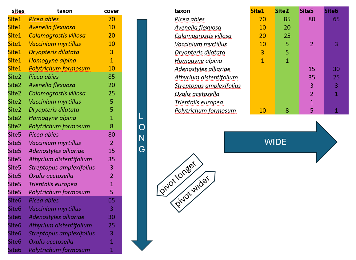
Wide format is more conservative and used in many older packages for ecological data analysis. In our example, we list all species, and the columns are used to indicate their abundance at each site. This is the way you need to prepare your species matrix for ordinations in vegan. However, wide format also has many cons.
One of them is the file size. In the example above, there is an abundance of given plants in each of the sites. When a species is present at only one site, such as Trientalis europaea, it still occupies space across the entire table, where there can be hundreds or thousands of sites. The table code, of course, is memory-demanding.
One more point. For many ecological analyses, you cannot keep the empty cells empty, since they are recognised as NAs. Therefore, you must take an additional step and fill them with zeros.
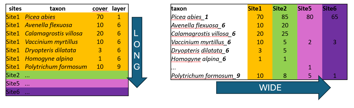
Another disadvantage is that it is not easy to add new information to the listed species. For example, if you want to separate species that are in a tree vegetation layer (recognised in vegetation ecology as 1), a herb layer (6), and a moss layer (9), you would have to add this information to the species name, e.g., Picea_abies_1. Can you see a conflict with the basic principles of tidyverse?
Long format, in contrast, is excellent for handling large datasets. Imagine we have more sites than those shown in the example above. In this format, we list all the species for Site1, then for Site2, and so on. However, we list only the species that are actually present! By simply counting the rows belonging to each site, you have the information about the overall species richness.
We can also add any information that describes the data, such as vegetation layers, growth forms, native/alien status, etc. After that, we can very simply filter, summarise and calculate further statistics.
4.2 From long to wide
We will first start a new script for this chapter and load the libraries. Remember to keep the script tidy and include your remarks.
Now, we will import the data. In the first example, we will again use the Forest understory data from our folder: Link to Github folder. However, this time we will upload the species data saved in a long format, and we will prepare a species matrix in a wide format, so that it can be used in specific ecological analyses, e.g. in vegan.
spe <- read_excel("data/forest_understory/Axmanova-Forest-spe.xlsx")
tibble(spe)
# A tibble: 2,277 × 4
RELEVE_NR Species Layer CoverPerc
<dbl> <chr> <dbl> <dbl>
1 1 Quercus petraea agg. 1 63
2 1 Acer campestre 1 18
3 1 Crataegus laevigata 4 2
4 1 Cornus mas 4 8
5 1 Lonicera xylosteum 4 3
6 1 Galium sylvaticum 6 3
7 1 Carex digitata 6 3
8 1 Melica nutans 6 2
9 1 Polygonatum odoratum 6 2
10 1 Geum urbanum 6 2
# ℹ 2,267 more rowsWe can see that there are plant species names sorted by RELEVE_NR, where each number indicates a vegetation record from a specific site (also known as a vegetation plot or sample). We will rename this to make it easier for us as PlotID. Furthermore, we may need to modify the species names to conform to the compact format, using underscores instead of spaces. For this, we will use the mutate() function with str_replace() (for string replacement), specifying that an underscore should replace each space, and apply it directly to the original column.
spe %>%
  rename(PlotID = RELEVE_NR) %>%
  mutate(Species = str_replace_all(Species, " ", "_"))
# A tibble: 2,277 × 4
PlotID Species Layer CoverPerc
<dbl> <chr> <dbl> <dbl>
1 1 Quercus_petraea_agg. 1 63
2 1 Acer_campestre 1 18
3 1 Crataegus_laevigata 4 2
4 1 Cornus_mas 4 8
5 1 Lonicera_xylosteum 4 3
6 1 Galium_sylvaticum 6 3
7 1 Carex_digitata 6 3
8 1 Melica_nutans 6 2
9 1 Polygonatum_odoratum 6 2
10 1 Geum_urbanum 6 2
# ℹ 2,267 more rows*If you want to play a bit, you can create a new column (e.g. SpeciesNew) to see both the original name and the changed name.
spe %>%
  rename(PlotID = RELEVE_NR) %>%
  mutate(SpeciesNew = str_replace_all(Species, " ", "_"))
# A tibble: 2,277 × 5
PlotID Species Layer CoverPerc SpeciesNew
<dbl> <chr> <dbl> <dbl> <chr>
1 1 Quercus petraea agg. 1 63 Quercus_petraea_agg.
2 1 Acer campestre 1 18 Acer_campestre
3 1 Crataegus laevigata 4 2 Crataegus_laevigata
4 1 Cornus mas 4 8 Cornus_mas
5 1 Lonicera xylosteum 4 3 Lonicera_xylosteum
6 1 Galium sylvaticum 6 3 Galium_sylvaticum
7 1 Carex digitata 6 3 Carex_digitata
8 1 Melica nutans 6 2 Melica_nutans
9 1 Polygonatum odoratum 6 2 Polygonatum_odoratum
10 1 Geum urbanum 6 2 Geum_urbanum
# ℹ 2,267 more rowsNote that, just as above, you can change different patterns, e.g., remove part of the strings. There are even more complex things we can do, but we will save them for later, as they require some knowledge of regular expression rules. Here, I created a new column where I removed the indication that the species belongs to a complex, i.e., the part of the string saying it is an aggregate. I also prepared a column “check” where I compare the new and old names to determine if they are equal or not, and filtered only those cases where they are not. This should show me exactly the changed rows. If I am satisfied with the result, I can then remove the lines using this check and even rewrite the original column.
spe %>%
  rename(PlotID = RELEVE_NR) %>%
  mutate(SpeciesNew = str_replace_all(Species, " agg.", "")) %>%
  mutate(check = (SpeciesNew == Species))%>%
  filter(check == "FALSE") %>%
  select(PlotID, Species, SpeciesNew, check) #select only relevant to see at a first glance
# A tibble: 159 × 4
PlotID Species SpeciesNew check
<dbl> <chr> <chr> <lgl>
1 1 Quercus petraea agg. Quercus petraea FALSE
2 1 Rubus fruticosus agg. Rubus fruticosus FALSE
3 1 Quercus petraea agg. Quercus petraea FALSE
4 2 Quercus petraea agg. Quercus petraea FALSE
5 2 Quercus petraea agg. Quercus petraea FALSE
6 3 Quercus petraea agg. Quercus petraea FALSE
7 3 Quercus petraea agg. Quercus petraea FALSE
8 3 Galium pumilum agg. Galium pumilum FALSE
9 3 Senecio nemorensis agg. Senecio nemorensis FALSE
10 3 Veronica chamaedrys agg. Veronica chamaedrys FALSE
# ℹ 149 more rowsWe have the condensed name with underscores, but there are still more variables in the table. We can either remove them or merge them to be included in the final wide format. Here, we will deviate slightly from tidy rules and add the information about the vegetation layer directly to the variable Species using the unite() function from the tidyr package, which merges strings from two or more columns into a new one: A+B = A_B. Default separator is again underscore, unless you specify it differently by the sep argument.
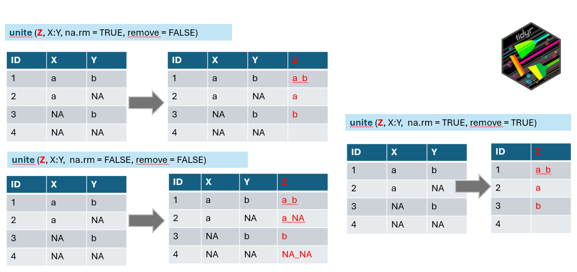 Argument
 na.rm indicates what to do if in one of the combined columns there is no value but NA. We have set this argument to TRUE to remove the NA. If you keep it FALSE, it is possible that in some data, the new string will be a_NA or NA_b, or even NA_NA (see line 4 of our example).
The remove argument set to TRUE will remove the original columns that we used to combine the new one (in the example above, you will have only z). In our case, we will keep the original columns for visual checking, and we will use the select() function in the next step to remove them.
Note that the function that works in the opposite direction is called separate() or separate_wider_delim().
spe %>%
  rename(PlotID = RELEVE_NR) %>%
  mutate(Species = str_replace_all(Species, " ", "_")) %>%
  unite("SpeciesLayer", Species, Layer, na.rm = TRUE, remove = FALSE)
# A tibble: 2,277 × 5
PlotID SpeciesLayer Species Layer CoverPerc
<dbl> <chr> <chr> <dbl> <dbl>
1 1 Quercus_petraea_agg._1 Quercus_petraea_agg. 1 63
2 1 Acer_campestre_1 Acer_campestre 1 18
3 1 Crataegus_laevigata_4 Crataegus_laevigata 4 2
4 1 Cornus_mas_4 Cornus_mas 4 8
5 1 Lonicera_xylosteum_4 Lonicera_xylosteum 4 3
6 1 Galium_sylvaticum_6 Galium_sylvaticum 6 3
7 1 Carex_digitata_6 Carex_digitata 6 3
8 1 Melica_nutans_6 Melica_nutans 6 2
9 1 Polygonatum_odoratum_6 Polygonatum_odoratum 6 2
10 1 Geum_urbanum_6 Geum_urbanum 6 2
# ℹ 2,267 more rowsAt this point, we have everything we need to use it as input for the wide-format table: PlotID, SpeciesLayer, and the values of abundance saved as CoverPerc. One more step is to select only these or deselect (-) those that are not needed.
spe %>%
  rename(PlotID = RELEVE_NR) %>%
  mutate(Species = str_replace_all(Species, " ", "_")) %>%
  unite("SpeciesLayer", Species, Layer, na.rm = TRUE, remove = FALSE) %>%
  select(PlotID, Species, Layer)
# A tibble: 2,277 × 3
PlotID Species Layer
<dbl> <chr> <dbl>
1 1 Quercus_petraea_agg. 1
2 1 Acer_campestre 1
3 1 Crataegus_laevigata 4
4 1 Cornus_mas 4
5 1 Lonicera_xylosteum 4
6 1 Galium_sylvaticum 6
7 1 Carex_digitata 6
8 1 Melica_nutans 6
9 1 Polygonatum_odoratum 6
10 1 Geum_urbanum 6
# ℹ 2,267 more rowsNow we can finally use the pivot_wider() function to transform the data. We need to specify where we are obtaining the names of new variables (names_from) and where we should get the values that should appear in the table (values_from).
spe %>%
  rename(PlotID = RELEVE_NR) %>%
  mutate(Species = str_replace_all(Species, " ", "_")) %>%
  unite("SpeciesLayer", Species, Layer, na.rm = TRUE, remove = TRUE) %>%
  pivot_wider(names_from = SpeciesLayer, values_from = CoverPerc)
# A tibble: 65 × 370
PlotID Quercus_petraea_agg._1 Acer_campestre_1 Crataegus_laevigata_4
<dbl> <dbl> <dbl> <dbl>
1 1 63 18 2
2 2 63 NA NA
3 3 63 NA NA
4 4 38 NA NA
5 5 63 NA NA
6 6 38 NA NA
7 7 63 NA NA
8 8 38 NA NA
9 9 38 NA NA
10 10 63 NA NA
# ℹ 55 more rows
# ℹ 366 more variables: Cornus_mas_4 <dbl>, Lonicera_xylosteum_4 <dbl>,
# Galium_sylvaticum_6 <dbl>, Carex_digitata_6 <dbl>, Melica_nutans_6 <dbl>,
# Polygonatum_odoratum_6 <dbl>, Geum_urbanum_6 <dbl>,
# Anemone_species_6 <dbl>, Viola_mirabilis_6 <dbl>,
# Hieracium_murorum_6 <dbl>, Platanthera_bifolia_6 <dbl>,
# Convallaria_majalis_6 <dbl>, Hepatica_nobilis_6 <dbl>, …There are different combinations of species in each plot, with some species present and others absent. Since we changed the format, all species, even those not occurring at that particular site or plot, must have some values. In long format, abundance or other information is not stored for absent species, so they are assigned NAs. Therefore, one additional step is to fill the empty cells with zeros using values_fill. In this case, we can do that because we know that if the species were absent, its abundance was exactly 0.
spe %>%
  rename(PlotID = RELEVE_NR) %>%
  mutate(Species = str_replace_all(Species, " ", "_")) %>%
  unite("SpeciesLayer", Species, Layer, na.rm = TRUE, remove = TRUE) %>%
  pivot_wider(names_from = SpeciesLayer, values_from = CoverPerc,
              values_fill = 0) -> spe_wide
4.3 From wide to long
Sometimes, it is necessary to transform data from wide to long format. Here, we need to say which column should not be changed, which is the PlotID (cols = -PlotID). Alternatively, -1 would also work.
Then we specify what to do with the column names, how they should be saved (names_to). And how to call the column with values (values_to).
spe_wide %>%
  pivot_longer(cols = -PlotID, names_to = 'species', values_to = 'cover')
# A tibble: 23,985 × 3
PlotID species cover
<dbl> <chr> <dbl>
1 1 Quercus_petraea_agg._1 63
2 1 Acer_campestre_1 18
3 1 Crataegus_laevigata_4 2
4 1 Cornus_mas_4 8
5 1 Lonicera_xylosteum_4 3
6 1 Galium_sylvaticum_6 3
7 1 Carex_digitata_6 3
8 1 Melica_nutans_6 2
9 1 Polygonatum_odoratum_6 2
10 1 Geum_urbanum_6 2
# ℹ 23,975 more rowsWe need to remove the empty rows. Since we previously filled them with zeros, we will first complete the transformation and then filter out the rows with a cover equal to zero.
spe_wide %>%
  pivot_longer(cols = -PlotID, names_to = 'species', values_to = 'cover') %>%
  filter(!cover == 0)
# A tibble: 2,277 × 3
PlotID species cover
<dbl> <chr> <dbl>
1 1 Quercus_petraea_agg._1 63
2 1 Acer_campestre_1 18
3 1 Crataegus_laevigata_4 2
4 1 Cornus_mas_4 8
5 1 Lonicera_xylosteum_4 3
6 1 Galium_sylvaticum_6 3
7 1 Carex_digitata_6 3
8 1 Melica_nutans_6 2
9 1 Polygonatum_odoratum_6 2
10 1 Geum_urbanum_6 2
# ℹ 2,267 more rowsSometimes, we have data with NAs (not zeros). Here, it is very useful to use argument values_drop_na= TRUE.
spe_wide %>%
  pivot_longer(cols = -PlotID, names_to = 'species', values_to = 'cover', values_drop_na = TRUE)
# A tibble: 23,985 × 3
PlotID species cover
<dbl> <chr> <dbl>
1 1 Quercus_petraea_agg._1 63
2 1 Acer_campestre_1 18
3 1 Crataegus_laevigata_4 2
4 1 Cornus_mas_4 8
5 1 Lonicera_xylosteum_4 3
6 1 Galium_sylvaticum_6 3
7 1 Carex_digitata_6 3
8 1 Melica_nutans_6 2
9 1 Polygonatum_odoratum_6 2
10 1 Geum_urbanum_6 2
# ℹ 23,975 more rows4.4 group_by(), count()
Using the group_by() function, we can define how the data should be arranged into groups. Then we can proceed with asking questions about these groups. The basic function of summarising information is to count the number of rows.
In the first example, we are working with a species list in a long format. We can easily calculate the number of species in each plot/sample by counting the corresponding number of rows. First, you have to specify what the grouping variable is. In this case, it would be PlotID. And then you can directly count.
spe %>%
  rename(PlotID = RELEVE_NR) %>%
  group_by(PlotID) %>%
  count()
# A tibble: 65 × 2
# Groups: PlotID [65]
PlotID n
<dbl> <int>
1 1 44
2 2 17
3 3 16
4 4 22
5 5 15
6 6 22
7 7 23
8 8 24
9 9 28
10 10 19
# ℹ 55 more rowscount() returns the number of rows in a new variable called n. You can directly put an extra line in your code and rename it. e.g. rename(SpeciesRichness = n). Note that in this case, we simply counted all the rows. However, we know that some woody species may be recorded in the tree vegetation layer as shrubs or as small juveniles, so we potentially calculated such species three times. We can experiment with the distinct() function and remove the layer information. Is there a difference in the resulting numbers?
spe %>%
  distinct(PlotID = RELEVE_NR, Species) %>%
  group_by(PlotID) %>%
  count() %>%
  rename(SpeciesRichness = n)
# A tibble: 65 × 2
# Groups: PlotID [65]
PlotID SpeciesRichness
<dbl> <int>
1 1 42
2 2 16
3 3 15
4 4 20
5 5 14
6 6 19
7 7 22
8 8 23
9 9 22
10 10 18
# ℹ 55 more rowsThe count() function can also be used in other cases. For example, we are interested in how many rows/plots/samples in the table are assigned to vegetation types. We will upload a table with descriptive characteristics for each forest plot, named env, which is a shortcut often used for an environmental data file.
env <- read_excel("data/forest_understory/Axmanova-Forest-env.xlsx")
tibble(env)
# A tibble: 65 × 13
RELEVE_NR ForestType ForestTypeName Biomass pH_KCl Canopy_E3 Radiation Heat
<dbl> <dbl> <chr> <dbl> <dbl> <dbl> <dbl> <dbl>
1 1 2 oak hornbeam f… 12.8 5.28 80 0.881 0.857
2 2 1 oak forest 9.9 3.24 80 0.933 0.814
3 3 1 oak forest 15.2 4.01 80 0.916 0.850
4 4 1 oak forest 16 3.76 75 0.930 0.948
5 5 1 oak forest 20.7 3.50 70 0.869 0.869
6 6 1 oak forest 46.4 3.8 65 0.918 0.883
7 7 1 oak forest 49.2 3.48 65 0.829 0.803
8 8 2 oak hornbeam f… 48.7 3.68 85 0.869 0.869
9 9 2 oak hornbeam f… 13.8 4.24 80 0.614 0.423
10 10 1 oak forest 79.1 4.00 70 0.905 0.930
# ℹ 55 more rows
# ℹ 5 more variables: TWI <dbl>, Longitude <dbl>, Latitude <dbl>,
# deg_lon <dbl>, deg_lat <dbl>And calculate the number of plots in each forest type.
env %>%
  group_by(ForestTypeName) %>%
  count()
# A tibble: 4 × 2
# Groups: ForestTypeName [4]
ForestTypeName n
<chr> <int>
1 alluvial forest 11
2 oak forest 16
3 oak hornbeam forest 28
4 ravine forest 10We can even skip the group_by() step and directly specify what to count, which is very useful.
env %>%
  count(ForestTypeName)
# A tibble: 4 × 2
ForestTypeName n
<chr> <int>
1 alluvial forest 11
2 oak forest 16
3 oak hornbeam forest 28
4 ravine forest 10The count() function can be very useful for checking duplicate rows. You can ask to count, for example, IDs in the file where you expect a unique ID in each row and filter those results that have more occurrences than 1. In the example below, each ID was used just once, so the filter returns no rows. Such a check is especially important if you need to append additional information using join functions.
env %>%
  count(PlotID = RELEVE_NR) %>%
  filter(n > 1)
# A tibble: 0 × 2
# ℹ 2 variables: PlotID <dbl>, n <int>4.5 summarise()
Using group_by() and summarise(), we can calculate, for example, the mean values or the total sum of values within a group. See more in the further reading. Here is an example of a summarise() for environmental data:
env %>%
  group_by(ForestTypeName) %>%
  summarise(meanBiomass = mean(Biomass))
# A tibble: 4 × 2
ForestTypeName meanBiomass
<chr> <dbl>
1 alluvial forest 148.
2 oak forest 26.7
3 oak hornbeam forest 44.4
4 ravine forest 79.1summarise() is also very useful for species data. For example, we can calculate the total abundance, approximated as cover, of all plants in the plot/sample. Later on, we can ask about the relative share of parasites, endangered species, or alien species. Alternatively, we can calculate the community mean of specific traits, such as the mean height of the plants or their mean leaf area index. For this, we would have to append new information so that we can leave it for the next chapter.
spe %>%
  group_by(PlotID = RELEVE_NR) %>%
  summarise(totalCover = sum(CoverPerc))
# A tibble: 65 × 2
PlotID totalCover
<dbl> <dbl>
1 1 164
2 2 115
3 3 101
4 4 96
5 5 109
6 6 121
7 7 147
8 8 185
9 9 128
10 10 174
# ℹ 55 more rowsWe can also define more variables we want to summarise and more functions we want to apply. Try to find out more here. Below is an example of the iris dataset, where we calculated the minimum, mean, and maximum values for sepal length and width in different species.
glimpse(iris)Rows: 150
Columns: 5
$ Sepal.Length <dbl> 5.1, 4.9, 4.7, 4.6, 5.0, 5.4, 4.6, 5.0, 4.4, 4.9, 5.4, 4.…
$ Sepal.Width <dbl> 3.5, 3.0, 3.2, 3.1, 3.6, 3.9, 3.4, 3.4, 2.9, 3.1, 3.7, 3.…
$ Petal.Length <dbl> 1.4, 1.4, 1.3, 1.5, 1.4, 1.7, 1.4, 1.5, 1.4, 1.5, 1.5, 1.…
$ Petal.Width <dbl> 0.2, 0.2, 0.2, 0.2, 0.2, 0.4, 0.3, 0.2, 0.2, 0.1, 0.2, 0.…
$ Species <fct> setosa, setosa, setosa, setosa, setosa, setosa, setosa, s…iris %>%
group_by(Species) %>%
summarise(across(c(Sepal.Length, Sepal.Width), list(min = min, mean = mean, max = max)))# A tibble: 3 × 7
Species Sepal.Length_min Sepal.Length_mean Sepal.Length_max Sepal.Width_min
<fct> <dbl> <dbl> <dbl> <dbl>
1 setosa 4.3 5.01 5.8 2.3
2 versicolor 4.9 5.94 7 2
3 virginica 4.9 6.59 7.9 2.2
# ℹ 2 more variables: Sepal.Width_mean <dbl>, Sepal.Width_max <dbl>4.6 Exercises
1. Forest Understory Data - download the data from the repository (Link to Github folder) and save it into your project folder. This dataset is used in the chapter above; please use it to prepare your own script with remarks, copy, and train what is described above. Note that you will use species data in long format: Axmanova-Forest-spe.xlsx, and environmental data Axmanova-Forest-env.xlsx
2. Use the Spruce forest data used in the graphical example at the beginning of this chapter. 2a, Import spruce_forestWIDE.xlsx > transform wide to long format > keep only true presences > calculate species richness for each site (count of number of species). 2b, Import also spruce_forestLONG.xlsx > and transform long to wide format.
3. Train the transformation of wide to long with another dataset, Acidophilous grasslands, namely the species file called SW_moravia_acidgrass_species.csv. Import the data and check the structure. Then, transform the format to long and remove absences. *Use the separate_wider_delim() function to separate information about the species name and layer into two variables.
4. Work with the dataset Lepidoptera, namely spe_matrix_MSvejnoha, which is the species file with counts of moths in forest steppe localities. Import the data and check the structure > transform to long format > count number of individuals at each site > create barplot to visualise the differences (ggplot2, geom_col). *For comparison, you can calculate the number of species (unique names) and visualise this as well.
5. Use Forest understory environmental data Axmanova-Forest-env.xlsx> prepare a new variable which will combine Forest type code and name (unite) > calculate mean values of biomass for these forest types (group_by, summarise) > prepare a graph with boxplots of forest type and biomass (ggplot2, geom_boxplot). *You can also play more with the data, calculate min, mean and max values for biomass and soil pH at once.
6. We will use the iris dataset integrated in R. Use glimpse(iris) to check the structure > if needed, change the format to tibble using the as_tibble() function (iris.data <- iris %>% as_tibble()) > calculate median values for selected parameters within different iris species.
7. “Tidy datasets are all alike, but every messy dataset is messy in its own way.” Hadley Wickham
Import Example4 from the messy_data and try to find duplicate rows.
8. * Import Example2 from the Messy data and try to make the data tidy with the use of the separate() function. This works in an opposite direction to unite().
4.7 Further reading
Summarise: https://dplyr.tidyverse.org/reference/summarise.html
Summarise multiple columns: https://dplyr.tidyverse.org/reference/summarise_all.html
Data transformation in R for Data Science: https://r4ds.hadley.nz/data-transform.html
Data tidying, including pivoting: https://r4ds.hadley.nz/data-tidy.html