library(palmerpenguins)
library(broom)
library(tidyverse)7 + 8 Automatisation
“Copy-and-paste is a powerful tool, but you should avoid doing it more than twice.” – Hadley Wickham, R for Data Science
It’s not only a matter of the script length. Repeating the same code multiple times might easily lead to errors and inconsistencies, and it is therefore better to avoid it. There are multiple ways to reduce copy-pasting when we want to repeat a similar operation multiple times. In this chapter, you will learn how to write your own function and some tools for iteration, including for loops and functions from the purrr package.
Throughout this chapter, we will use the following packages:
7.1 Functions
In more complex data analysis tasks, when you need to repeat a similar operation multiple times, e.g. calculate the same model for multiple subsets of data, calculate models with the same explanatory variables for different response variables, or draw similarly looking plots for multiple variables, it becomes really useful to be able to write your own function and hide the repeated code into it. A huge advantage of only writing the code once and saving it as a function is that when you have to change something, you only do it once and thus prevent mistakes like replacing the variable name in one place but not in the other, etc. In the long term, it also saves time and improves the understandability of the code, as the script does not end up being hundreds or thousands of lines long and all important commands are in one place.
We will use a penguin dataset that you know already:
glimpse(penguins)Rows: 344
Columns: 8
$ species <fct> Adelie, Adelie, Adelie, Adelie, Adelie, Adelie, Adel…
$ island <fct> Torgersen, Torgersen, Torgersen, Torgersen, Torgerse…
$ bill_length_mm <dbl> 39.1, 39.5, 40.3, NA, 36.7, 39.3, 38.9, 39.2, 34.1, …
$ bill_depth_mm <dbl> 18.7, 17.4, 18.0, NA, 19.3, 20.6, 17.8, 19.6, 18.1, …
$ flipper_length_mm <int> 181, 186, 195, NA, 193, 190, 181, 195, 193, 190, 186…
$ body_mass_g <int> 3750, 3800, 3250, NA, 3450, 3650, 3625, 4675, 3475, …
$ sex <fct> male, female, female, NA, female, male, female, male…
$ year <int> 2007, 2007, 2007, 2007, 2007, 2007, 2007, 2007, 2007…7.1.1 Vector functions
Let’s say we want to standardise each measured variable in the dataset, and just imagine for now that there is no scale() function, so we have to do it manually. We would end up with something like this:
penguins |>
  mutate(bill_length_mm = (bill_length_mm - mean(bill_length_mm, na.rm = T))/sd(bill_length_mm, na.rm = T),
         bill_depth_mm = (bill_depth_mm - mean(bill_depth_mm, na.rm = T))/sd(bill_depth_mm, na.rm = T),
         flipper_length_mm = (flipper_length_mm - mean(flipper_length_mm, na.rm = T))/sd(flipper_length_mm, na.rm = T),
         body_mass_g = (body_mass_g - mean(body_mass_g, na.rm = T))/sd(body_mass_g, na.rm = T))
# A tibble: 344 × 8
species island bill_length_mm bill_depth_mm flipper_length_mm body_mass_g
<fct> <fct> <dbl> <dbl> <dbl> <dbl>
1 Adelie Torgersen -0.883 0.784 -1.42 -0.563
2 Adelie Torgersen -0.810 0.126 -1.06 -0.501
3 Adelie Torgersen -0.663 0.430 -0.421 -1.19
4 Adelie Torgersen NA NA NA NA
5 Adelie Torgersen -1.32 1.09 -0.563 -0.937
6 Adelie Torgersen -0.847 1.75 -0.776 -0.688
7 Adelie Torgersen -0.920 0.329 -1.42 -0.719
8 Adelie Torgersen -0.865 1.24 -0.421 0.590
9 Adelie Torgersen -1.80 0.480 -0.563 -0.906
10 Adelie Torgersen -0.352 1.54 -0.776 0.0602
# ℹ 334 more rows
# ℹ 2 more variables: sex <fct>, year <int>When creating such a code, it is quite easy to forget to replace the variable name in one place when copying it. To avoid that and make the code easier to read, we can transform the code into a function. We need three things to do that:
- a function name, this should be concise and informative (please avoid
myfunction1(), etc.) and not mess up already existing functions, we will usecustom_scaleto distinguish our function from thescale(). - arguments, which are the things that we want to vary across calls, in our case, we have just one numerical variable we are working with, so we will call it
x. - body, that is the code that stays the same across calls.
Every function defined in R has the following structure:
name <- function(arguments){
  body
}
In our case, the function would look like this:
custom_scale <- function(x){
  (x - mean(x, na.rm = T))/sd(x, na.rm = T)
}
When we run this code, our new function is saved into the environment, and we can use it as any other function. We created a function that takes a vector and returns a vector of the same length that might be use within the mutate() function.
penguins |>
  mutate(bill_length_mm = custom_scale(bill_length_mm),
         bill_depth_mm = custom_scale(bill_depth_mm),
         flipper_length_mm = custom_scale(flipper_length_mm),
         body_mass_g = custom_scale(body_mass_g))
# A tibble: 344 × 8
species island bill_length_mm bill_depth_mm flipper_length_mm body_mass_g
<fct> <fct> <dbl> <dbl> <dbl> <dbl>
1 Adelie Torgersen -0.883 0.784 -1.42 -0.563
2 Adelie Torgersen -0.810 0.126 -1.06 -0.501
3 Adelie Torgersen -0.663 0.430 -0.421 -1.19
4 Adelie Torgersen NA NA NA NA
5 Adelie Torgersen -1.32 1.09 -0.563 -0.937
6 Adelie Torgersen -0.847 1.75 -0.776 -0.688
7 Adelie Torgersen -0.920 0.329 -1.42 -0.719
8 Adelie Torgersen -0.865 1.24 -0.421 0.590
9 Adelie Torgersen -1.80 0.480 -0.563 -0.906
10 Adelie Torgersen -0.352 1.54 -0.776 0.0602
# ℹ 334 more rows
# ℹ 2 more variables: sex <fct>, year <int>We can, of course, reduce the duplication even further by using the across() function:
penguins |>
  mutate(across(c(bill_length_mm, bill_depth_mm, flipper_length_mm, body_mass_g), ~custom_scale(.x)))
# A tibble: 344 × 8
species island bill_length_mm bill_depth_mm flipper_length_mm body_mass_g
<fct> <fct> <dbl> <dbl> <dbl> <dbl>
1 Adelie Torgersen -0.883 0.784 -1.42 -0.563
2 Adelie Torgersen -0.810 0.126 -1.06 -0.501
3 Adelie Torgersen -0.663 0.430 -0.421 -1.19
4 Adelie Torgersen NA NA NA NA
5 Adelie Torgersen -1.32 1.09 -0.563 -0.937
6 Adelie Torgersen -0.847 1.75 -0.776 -0.688
7 Adelie Torgersen -0.920 0.329 -1.42 -0.719
8 Adelie Torgersen -0.865 1.24 -0.421 0.590
9 Adelie Torgersen -1.80 0.480 -0.563 -0.906
10 Adelie Torgersen -0.352 1.54 -0.776 0.0602
# ℹ 334 more rows
# ℹ 2 more variables: sex <fct>, year <int>There are some useful RStudio keyboard shortcuts you can use to work with functions:
To find a definition of any function, place a cursor on the name of the function in the script and press
F2.To extract a function from a code you have written, use
Alt + Ctrl + X. Just be sure you always check the results, because sometimes it will not do exactly what you expect, so you will have to make some adjustments.
We can also write summary functions to be used in a summarise() call. For example, we could calculate the difference between the minimum and maximum values of the given variable:
range_diff <- function(x){
  max(x, na.rm = T) - min(x, na.rm = T)
}

penguins |>
  summarize(bill_length_mm = range_diff(bill_length_mm),
            bill_depth_mm = range_diff(bill_depth_mm))
# A tibble: 1 × 2
bill_length_mm bill_depth_mm
<dbl> <dbl>
1 27.5 8.47.1.2 Data frame functions
Till now, we have written several vector functions that might be used within dplyr functions. But functions may operate even at the data frame level. We will show here a real-world example of data sampled in three types of sand vegetation - pioneer sand vegetation (Corynephorion), acidophilous sand grasslands (Armerion) and basiphilous sand grasslands (Festucion valesiacae). The species data of all three vegetation types are saved in a long format in one file, and the header data with cluster assignment in a second file.
spe_long <- read_csv('data/sands/sands_spe_long.csv')Rows: 3154 Columns: 3
── Column specification ────────────────────────────────────────────────────────
Delimiter: ","
chr (1): valid_name
dbl (2): releve_nr, cover_perc
ℹ Use `spec()` to retrieve the full column specification for this data.
ℹ Specify the column types or set `show_col_types = FALSE` to quiet this message.glimpse(spe_long)Rows: 3,154
Columns: 3
$ releve_nr <dbl> 1, 1, 1, 1, 1, 1, 1, 1, 1, 1, 1, 1, 1, 2, 2, 2, 2, 2, 2, 2,…
$ valid_name <chr> "Achillea millefolium agg.", "Artemisia campestris", "Carex…
$ cover_perc <dbl> 0.5, 0.5, 0.5, 3.0, 0.5, 15.0, 0.5, 0.5, 0.5, 0.5, 0.5, 0.5…head <- read_csv('data/sands/sands_head.csv') |>
select(releve_nr, cluster)Rows: 172 Columns: 89
── Column specification ────────────────────────────────────────────────────────
Delimiter: ","
chr (40): country, reference, nr_in_tab, coverscale, author, syntaxon, moss_...
dbl (46): releve_nr, table_nr, date, surf_area, altitude, exposition, inclin...
lgl (3): rs_project, maniptyp, name_ass
ℹ Use `spec()` to retrieve the full column specification for this data.
ℹ Specify the column types or set `show_col_types = FALSE` to quiet this message.glimpse(head)Rows: 172
Columns: 2
$ releve_nr <dbl> 1, 2, 3, 4, 6, 7, 8, 9, 10, 11, 12, 14, 15, 16, 17, 18, 19, …
$ cluster <chr> "Corynephorion", "Armerion", "Corynephorion", "Corynephorion…Imagine we now want to run an ordination analysis that needs species data in a wide format for each of the three vegetation types separately. We need to subset the species data to only the selected vegetation type, select only relevant columns, square-root the species abundances, and transform the data into a wide format. We can incorporate all these steps into a single function, that we will then run three times for different subsets:
subset_to_wide <- function(data_long, veg_type){
  data_long |>
    semi_join(head |> filter(cluster == veg_type)) |>
    select(releve_nr, valid_name, cover_perc) |>
    mutate(cover_perc = sqrt(cover_perc)) |>
    pivot_wider(names_from = valid_name, values_from = cover_perc, values_fill = 0) |>
    select(-releve_nr)
}

spe_wide_cory <- subset_to_wide(spe_long, 'Corynephorion')
Joining with `by = join_by(releve_nr)`spe_wide_arm <- subset_to_wide(spe_long, 'Armerion')Joining with `by = join_by(releve_nr)`spe_wide_fes <- subset_to_wide(spe_long, 'Festucion valesiacae')Joining with `by = join_by(releve_nr)`Writing your own functions with the dplyr and tidyr calls inside sometimes also brings some challenges. We unfortunately do not have enough space here to deal with them, but there are great sources with detailed explanation, where you can learn more or find help if needed, e.g. https://r4ds.hadley.nz/functions.html#data-frame-functions, programming with dplyr, programming with tidyr, What is data-masking and why do I need {{?.
7.1.3 Plot functions
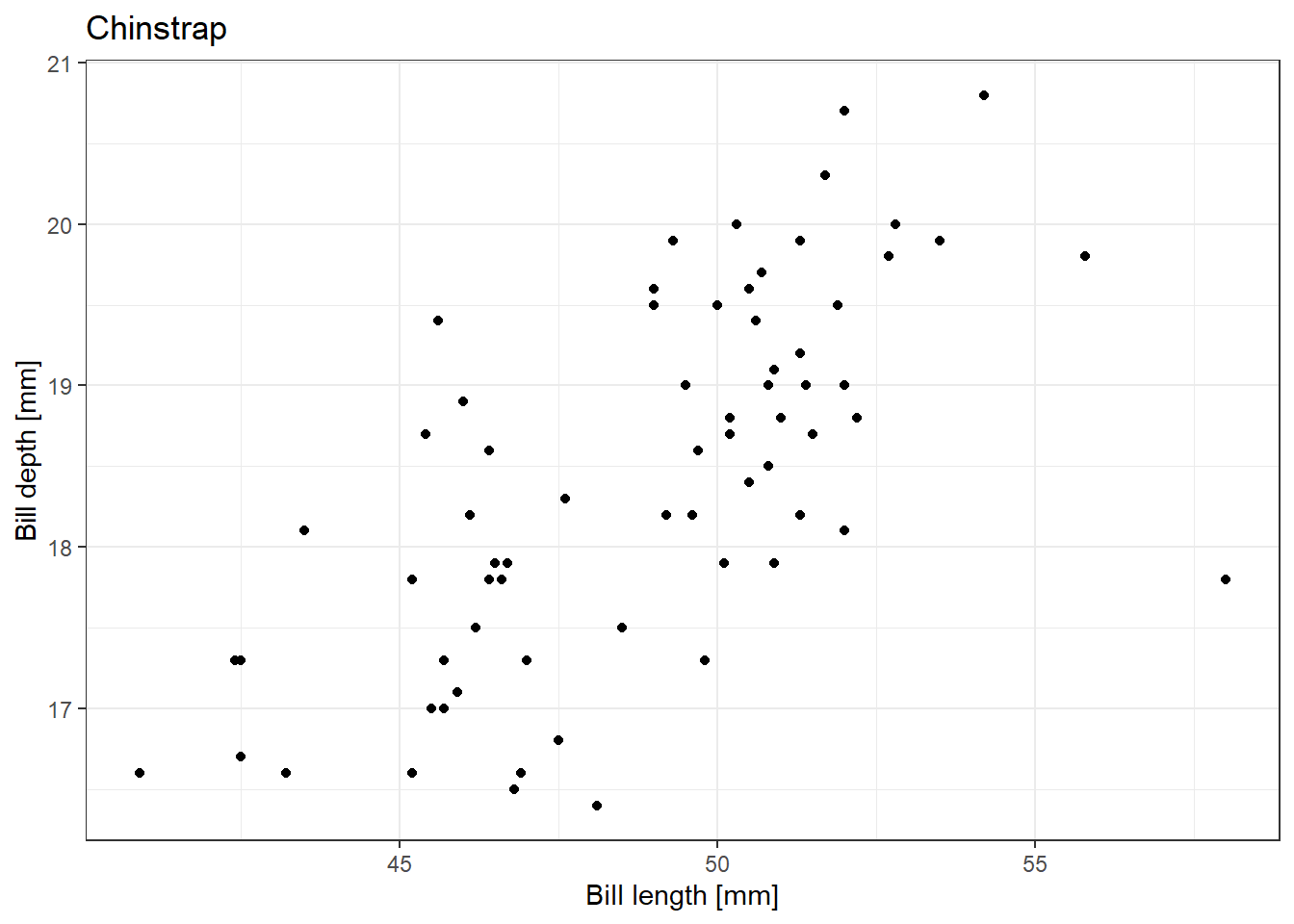
Sometimes it is also useful to reduce the amount of replicated code when plotting many different things in a similar way. The plot functions work similarly to the data frame functions, just return a plot instead of a data frame. For example, we might want to visualise the relationship between bill length and bill depth of three different penguin species separately. We have to first filter our penguin dataset to contain data on only one species, and then create a scatterplot using a ggplot sequence. This is how we would write the code for plotting the data for one species:
penguins |>
    filter(species == 'Adelie') |>
    ggplot(aes(bill_length_mm, bill_depth_mm)) +
    geom_point() +
    theme_bw() +
    labs(title = 'Adelie', x = 'Bill length [mm]', y = 'Bill depth [mm]')
Warning: Removed 1 row containing missing values or values outside the scale range
(`geom_point()`).
Let’s now turn this code into a function instead of copy-pasting it two more times to plot the same relationship for the two other species:
plot_species <- function(data, species_name){
data |>
filter(species == species_name) |>
ggplot(aes(bill_length_mm, bill_depth_mm)) +
geom_point() +
theme_bw() +
labs(title = species_name, x = 'Bill length [mm]', y = 'Bill depth [mm]')
}
plot_species(penguins, 'Adelie')Warning: Removed 1 row containing missing values or values outside the scale range
(`geom_point()`).
To learn more about reducing duplication in your ggplot2 code look here: https://r4ds.hadley.nz/functions.html#plot-functions, Programming with ggplot2, https://ggplot2.tidyverse.org/articles/ggplot2-in-packages.html.
7.2 For loops
We will now move to the iteration part of this chapter, which means repeating the same action multiple times on different objects. In any programming language, it is possible to automate such repetitions using a for loop. The basic structure of a for loop looks like this:
for (variable in sequence) {
# do something with the variable
}The for loop takes one variable from a given sequence, runs the code inside {} for this variable and then moves to the next variable in the sequence. A basic example might be printing numbers from a sequence:
for (i in 1:5) {
print(i)
}[1] 1
[1] 2
[1] 3
[1] 4
[1] 5The for loop takes one number, prints it, then takes the next one, prints it, and so on till the end of the sequence.
We can, for example, take our plot function to plot the scatterplot of bill length and bill depth of individual species and loop over the species names to sequentially make a plot for all species.
for (species_name in unique(penguins$species)) {
plot_species(penguins, species_name) |>
print()
}Warning: Removed 1 row containing missing values or values outside the scale range
(`geom_point()`).
Warning: Removed 1 row containing missing values or values outside the scale range
(`geom_point()`).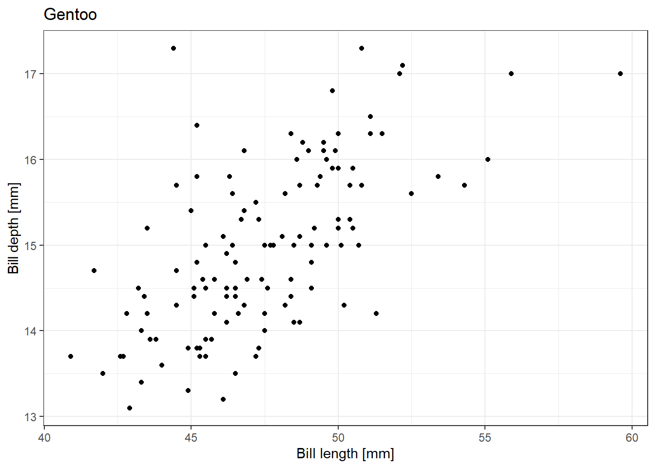
There are always multiple ways to get to the same result, and this is also true for iteration in R. The purrr package has powerful tools to iterate over multiple elements. Once the problems become more complex, it becomes more effective to use purrr functions in a pipeline instead of complicated nested for loops. But even when you choose to prefer purrr solutions, it is worth being familiar with for loops and their functionality, because you might see them often in the code of other people, and they are universal across programming languages.
7.3 purrr and working with nested dataframes
7.3.1 Basic usage of purrr
We already went through most of the tidyverse packages, but we didn’t talk about the purrr package yet. purrr provides powerful tools for automatisation of tasks that need to be repeated multiple times, e.g. for each file in a directory, each element of a list, each dataframe… They allow you to replace for loops with map() functions, which might be more powerful, readable and consistent with the rest of tidyverse.
The map() function works similarly to across(), but instead of applying a function to each column in a data frame or tibble, it applies a function to each element of a vector or list. It is an analogy of a for loop, the function takes each element of a sequence and applies a function to it. Let’s look at the difference between the for loop and map() in the following example:
# for loop
for (i in 1:5) {
  print(i)
}
[1] 1
[1] 2
[1] 3
[1] 4
[1] 5map(1:5, ~.x)[[1]]
[1] 1
[[2]]
[1] 2
[[3]]
[1] 3
[[4]]
[1] 4
[[5]]
[1] 5The structure of the map() function may already be familiar to you, as it resembles that of the across(). Note the difference between the output of the for loop and map(). In the output of the for loop, we see [1] 1, whereas map() returns [[1]] [1] 1. This is because the map() function returns a list. We can save the output to an object and look at the structure.
map_out <- map(1:5, ~.x)In the environment, you will see it is a list, we can also explore the structure using View(). The individual values inside the list are called using double square brackets e.g., map_out[[1]]. This might be helpful to remember for further work with lists and map() functions.
map_out[[1]][1] 1In addition to map(), purrr contains also several relatives, which return different output types:
map()makes a listmap_lgl()makes a logical vectormap_int()makes an integer vectormap_dbl()makes a double vectormap_chr()makes a character vector
Each of the above-mentioned functions takes a vector input, applies a function to each element and returns a vector of the same length.
map2()takes two vectors, usually of the same length and iterates over two arguments at a time
And there is also a group of walk() functions, which return their side-effects and return the input .x. They might be used, for example, for saving multiple files or plots.
We will now look at several examples of their usage. We can use the map() function to apply any function to multiple elements. It becomes very useful for working with lists. As a basic example, we can apply a simple function like sqrt() to every element of a list.
test_list <- list(2, 4, 6, 8, 10)

map(test_list, ~sqrt(.x))
[[1]]
[1] 1.414214
[[2]]
[1] 2
[[3]]
[1] 2.44949
[[4]]
[1] 2.828427
[[5]]
[1] 3.162278To get a numeric vector output, we can use the map_dbl() function.
map_dbl(test_list, ~sqrt(.x))[1] 1.414214 2.000000 2.449490 2.828427 3.162278And we can also write it with the pipe:
test_list |> map_dbl(~sqrt(.x))[1] 1.414214 2.000000 2.449490 2.828427 3.162278We can also rewrite our for loop used for creating plots of the relationship between penguin bill length and bill depth separately using the function from 7.1.3 in a map() function:
map(unique(penguins$species), ~plot_species(penguins, .x))[[1]]Warning: Removed 1 row containing missing values or values outside the scale range
(`geom_point()`).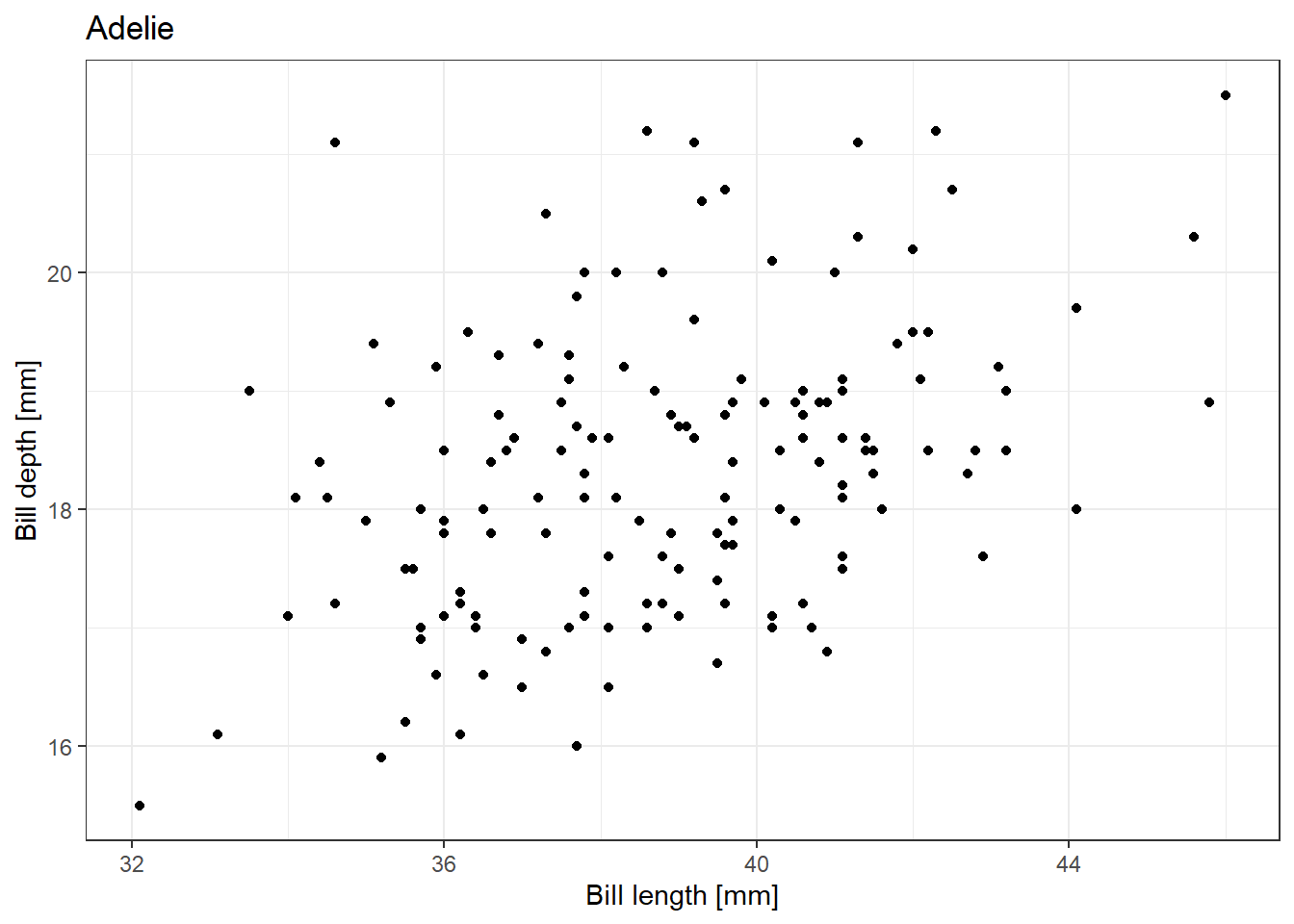
[[2]]Warning: Removed 1 row containing missing values or values outside the scale range
(`geom_point()`).
[[3]]
map2() takes two vectors or lists of the same length and iterates over them in pairs. We can illustrate this on the following example, where we will combine two lists with character strings in a single one:
genus <- list('Acer', 'Quercus', 'Tilia', 'Fagus')
species <- list('platanoides', 'petraea', 'cordata', 'sylvatica')

map2(genus, species, ~str_c(.x, .y, sep = ' '))
[[1]]
[1] "Acer platanoides"
[[2]]
[1] "Quercus petraea"
[[3]]
[1] "Tilia cordata"
[[4]]
[1] "Fagus sylvatica"The str_c() function from the stringr package combines two or more character strings in one, we specify the elements that should be combined and the separator that should be placed in between. Note that we now have two arguments to iterate over, and thus we must use two placeholders, .x and .y, where .x represents the first argument of map2() and .y represents the second. Similarly to map(), map2() also creates a list. We can add <- assignment and store the result in the environment and explore the structure.
genus_species <- map2(genus, species, ~str_c(.x, .y, sep = ' '))We can also use the relatives map2_dbl(), map2_chr() etc., to create a single vector. In the case of the species names the result is a character, so we will use map2_chr().
map2_chr(genus, species, ~str_c(.x, .y, sep = ' '))[1] "Acer platanoides" "Quercus petraea" "Tilia cordata" "Fagus sylvatica" 7.3.2 Loading multiple files
The huge advantage of such an approach becomes more visible once we start, e.g., working with multiple datasets with the same structure, building the same models for different variables, or plotting many plots.
Let’s begin with the task of reading multiple files simultaneously. Imagine you have multiple files with the same structure, but for some reason, they are stored in separate files. As example data, we will use the gapminder dataset, which provides values for life expectancy, GDP per capita, and population size. The data we have in the gapminder folder (Link to the Github folder) is divided by year
list.files('data/gapminder/') [1] "gapminder_1952.csv" "gapminder_1957.csv" "gapminder_1962.csv"
[4] "gapminder_1967.csv" "gapminder_1972.csv" "gapminder_1977.csv"
[7] "gapminder_1982.csv" "gapminder_1987.csv" "gapminder_1992.csv"
[10] "gapminder_1997.csv" "gapminder_2002.csv" "gapminder_2007.csv"We now want to load them all and combine them into a single tibble. We could do that by copy-pasting the read_csv() function twelve times, but there is a more elegant way. First, we will have to create a vector of paths to the individual files. In addition to what we know already, we added two more arguments to list.files(). pattern specifies a common pattern of the files we want to list, in our case .csv to ensure we will load only csv files in case there is some other file, e.g. a readme, in the folder. full.names = T returns a full path to the file from the project directory needed to read the file.
paths <- list.files('data/gapminder/', pattern = '.csv', full.names = T)
paths
[1] "data/gapminder/gapminder_1952.csv" "data/gapminder/gapminder_1957.csv"
[3] "data/gapminder/gapminder_1962.csv" "data/gapminder/gapminder_1967.csv"
[5] "data/gapminder/gapminder_1972.csv" "data/gapminder/gapminder_1977.csv"
[7] "data/gapminder/gapminder_1982.csv" "data/gapminder/gapminder_1987.csv"
[9] "data/gapminder/gapminder_1992.csv" "data/gapminder/gapminder_1997.csv"
[11] "data/gapminder/gapminder_2002.csv" "data/gapminder/gapminder_2007.csv"Now we can use the map() function to load all these datasets from a single line of code:
files <- map(paths, ~read_csv(.x))Rows: 142 Columns: 5
── Column specification ────────────────────────────────────────────────────────
Delimiter: ","
chr (2): country, continent
dbl (3): lifeExp, pop, gdpPercap
ℹ Use `spec()` to retrieve the full column specification for this data.
ℹ Specify the column types or set `show_col_types = FALSE` to quiet this message.
Rows: 142 Columns: 5
── Column specification ────────────────────────────────────────────────────────
Delimiter: ","
chr (2): country, continent
dbl (3): lifeExp, pop, gdpPercap
ℹ Use `spec()` to retrieve the full column specification for this data.
ℹ Specify the column types or set `show_col_types = FALSE` to quiet this message.We can now check the structure of object we just created:
str(files)List of 12
$ : spc_tbl_ [142 × 5] (S3: spec_tbl_df/tbl_df/tbl/data.frame)
..$ country : chr [1:142] "Afghanistan" "Albania" "Algeria" "Angola" ...
..$ continent: chr [1:142] "Asia" "Europe" "Africa" "Africa" ...
..$ lifeExp : num [1:142] 28.8 55.2 43.1 30 62.5 ...
..$ pop : num [1:142] 8425333 1282697 9279525 4232095 17876956 ...
..$ gdpPercap: num [1:142] 779 1601 2449 3521 5911 ...
..- attr(*, "spec")=
.. .. cols(
.. .. country = col_character(),
.. .. continent = col_character(),
.. .. lifeExp = col_double(),
.. .. pop = col_double(),
.. .. gdpPercap = col_double()
.. .. )
..- attr(*, "problems")=<externalptr>
$ : spc_tbl_ [142 × 5] (S3: spec_tbl_df/tbl_df/tbl/data.frame)
..$ country : chr [1:142] "Afghanistan" "Albania" "Algeria" "Angola" ...
..$ continent: chr [1:142] "Asia" "Europe" "Africa" "Africa" ...
..$ lifeExp : num [1:142] 30.3 59.3 45.7 32 64.4 ...
..$ pop : num [1:142] 9240934 1476505 10270856 4561361 19610538 ...
..$ gdpPercap: num [1:142] 821 1942 3014 3828 6857 ...
..- attr(*, "spec")=
.. .. cols(
.. .. country = col_character(),
.. .. continent = col_character(),
.. .. lifeExp = col_double(),
.. .. pop = col_double(),
.. .. gdpPercap = col_double()
.. .. )
..- attr(*, "problems")=<externalptr>
$ : spc_tbl_ [142 × 5] (S3: spec_tbl_df/tbl_df/tbl/data.frame)
..$ country : chr [1:142] "Afghanistan" "Albania" "Algeria" "Angola" ...
..$ continent: chr [1:142] "Asia" "Europe" "Africa" "Africa" ...
..$ lifeExp : num [1:142] 32 64.8 48.3 34 65.1 ...
..$ pop : num [1:142] 10267083 1728137 11000948 4826015 21283783 ...
..$ gdpPercap: num [1:142] 853 2313 2551 4269 7133 ...
..- attr(*, "spec")=
.. .. cols(
.. .. country = col_character(),
.. .. continent = col_character(),
.. .. lifeExp = col_double(),
.. .. pop = col_double(),
.. .. gdpPercap = col_double()
.. .. )
..- attr(*, "problems")=<externalptr>
$ : spc_tbl_ [142 × 5] (S3: spec_tbl_df/tbl_df/tbl/data.frame)
..$ country : chr [1:142] "Afghanistan" "Albania" "Algeria" "Angola" ...
..$ continent: chr [1:142] "Asia" "Europe" "Africa" "Africa" ...
..$ lifeExp : num [1:142] 34 66.2 51.4 36 65.6 ...
..$ pop : num [1:142] 11537966 1984060 12760499 5247469 22934225 ...
..$ gdpPercap: num [1:142] 836 2760 3247 5523 8053 ...
..- attr(*, "spec")=
.. .. cols(
.. .. country = col_character(),
.. .. continent = col_character(),
.. .. lifeExp = col_double(),
.. .. pop = col_double(),
.. .. gdpPercap = col_double()
.. .. )
..- attr(*, "problems")=<externalptr>
$ : spc_tbl_ [142 × 5] (S3: spec_tbl_df/tbl_df/tbl/data.frame)
..$ country : chr [1:142] "Afghanistan" "Albania" "Algeria" "Angola" ...
..$ continent: chr [1:142] "Asia" "Europe" "Africa" "Africa" ...
..$ lifeExp : num [1:142] 36.1 67.7 54.5 37.9 67.1 ...
..$ pop : num [1:142] 13079460 2263554 14760787 5894858 24779799 ...
..$ gdpPercap: num [1:142] 740 3313 4183 5473 9443 ...
..- attr(*, "spec")=
.. .. cols(
.. .. country = col_character(),
.. .. continent = col_character(),
.. .. lifeExp = col_double(),
.. .. pop = col_double(),
.. .. gdpPercap = col_double()
.. .. )
..- attr(*, "problems")=<externalptr>
$ : spc_tbl_ [142 × 5] (S3: spec_tbl_df/tbl_df/tbl/data.frame)
..$ country : chr [1:142] "Afghanistan" "Albania" "Algeria" "Angola" ...
..$ continent: chr [1:142] "Asia" "Europe" "Africa" "Africa" ...
..$ lifeExp : num [1:142] 38.4 68.9 58 39.5 68.5 ...
..$ pop : num [1:142] 14880372 2509048 17152804 6162675 26983828 ...
..$ gdpPercap: num [1:142] 786 3533 4910 3009 10079 ...
..- attr(*, "spec")=
.. .. cols(
.. .. country = col_character(),
.. .. continent = col_character(),
.. .. lifeExp = col_double(),
.. .. pop = col_double(),
.. .. gdpPercap = col_double()
.. .. )
..- attr(*, "problems")=<externalptr>
$ : spc_tbl_ [142 × 5] (S3: spec_tbl_df/tbl_df/tbl/data.frame)
..$ country : chr [1:142] "Afghanistan" "Albania" "Algeria" "Angola" ...
..$ continent: chr [1:142] "Asia" "Europe" "Africa" "Africa" ...
..$ lifeExp : num [1:142] 39.9 70.4 61.4 39.9 69.9 ...
..$ pop : num [1:142] 12881816 2780097 20033753 7016384 29341374 ...
..$ gdpPercap: num [1:142] 978 3631 5745 2757 8998 ...
..- attr(*, "spec")=
.. .. cols(
.. .. country = col_character(),
.. .. continent = col_character(),
.. .. lifeExp = col_double(),
.. .. pop = col_double(),
.. .. gdpPercap = col_double()
.. .. )
..- attr(*, "problems")=<externalptr>
$ : spc_tbl_ [142 × 5] (S3: spec_tbl_df/tbl_df/tbl/data.frame)
..$ country : chr [1:142] "Afghanistan" "Albania" "Algeria" "Angola" ...
..$ continent: chr [1:142] "Asia" "Europe" "Africa" "Africa" ...
..$ lifeExp : num [1:142] 40.8 72 65.8 39.9 70.8 ...
..$ pop : num [1:142] 13867957 3075321 23254956 7874230 31620918 ...
..$ gdpPercap: num [1:142] 852 3739 5681 2430 9140 ...
..- attr(*, "spec")=
.. .. cols(
.. .. country = col_character(),
.. .. continent = col_character(),
.. .. lifeExp = col_double(),
.. .. pop = col_double(),
.. .. gdpPercap = col_double()
.. .. )
..- attr(*, "problems")=<externalptr>
$ : spc_tbl_ [142 × 5] (S3: spec_tbl_df/tbl_df/tbl/data.frame)
..$ country : chr [1:142] "Afghanistan" "Albania" "Algeria" "Angola" ...
..$ continent: chr [1:142] "Asia" "Europe" "Africa" "Africa" ...
..$ lifeExp : num [1:142] 41.7 71.6 67.7 40.6 71.9 ...
..$ pop : num [1:142] 16317921 3326498 26298373 8735988 33958947 ...
..$ gdpPercap: num [1:142] 649 2497 5023 2628 9308 ...
..- attr(*, "spec")=
.. .. cols(
.. .. country = col_character(),
.. .. continent = col_character(),
.. .. lifeExp = col_double(),
.. .. pop = col_double(),
.. .. gdpPercap = col_double()
.. .. )
..- attr(*, "problems")=<externalptr>
$ : spc_tbl_ [142 × 5] (S3: spec_tbl_df/tbl_df/tbl/data.frame)
..$ country : chr [1:142] "Afghanistan" "Albania" "Algeria" "Angola" ...
..$ continent: chr [1:142] "Asia" "Europe" "Africa" "Africa" ...
..$ lifeExp : num [1:142] 41.8 73 69.2 41 73.3 ...
..$ pop : num [1:142] 22227415 3428038 29072015 9875024 36203463 ...
..$ gdpPercap: num [1:142] 635 3193 4797 2277 10967 ...
..- attr(*, "spec")=
.. .. cols(
.. .. country = col_character(),
.. .. continent = col_character(),
.. .. lifeExp = col_double(),
.. .. pop = col_double(),
.. .. gdpPercap = col_double()
.. .. )
..- attr(*, "problems")=<externalptr>
$ : spc_tbl_ [142 × 5] (S3: spec_tbl_df/tbl_df/tbl/data.frame)
..$ country : chr [1:142] "Afghanistan" "Albania" "Algeria" "Angola" ...
..$ continent: chr [1:142] "Asia" "Europe" "Africa" "Africa" ...
..$ lifeExp : num [1:142] 42.1 75.7 71 41 74.3 ...
..$ pop : num [1:142] 25268405 3508512 31287142 10866106 38331121 ...
..$ gdpPercap: num [1:142] 727 4604 5288 2773 8798 ...
..- attr(*, "spec")=
.. .. cols(
.. .. country = col_character(),
.. .. continent = col_character(),
.. .. lifeExp = col_double(),
.. .. pop = col_double(),
.. .. gdpPercap = col_double()
.. .. )
..- attr(*, "problems")=<externalptr>
$ : spc_tbl_ [142 × 5] (S3: spec_tbl_df/tbl_df/tbl/data.frame)
..$ country : chr [1:142] "Afghanistan" "Albania" "Algeria" "Angola" ...
..$ continent: chr [1:142] "Asia" "Europe" "Africa" "Africa" ...
..$ lifeExp : num [1:142] 43.8 76.4 72.3 42.7 75.3 ...
..$ pop : num [1:142] 31889923 3600523 33333216 12420476 40301927 ...
..$ gdpPercap: num [1:142] 975 5937 6223 4797 12779 ...
..- attr(*, "spec")=
.. .. cols(
.. .. country = col_character(),
.. .. continent = col_character(),
.. .. lifeExp = col_double(),
.. .. pop = col_double(),
.. .. gdpPercap = col_double()
.. .. )
..- attr(*, "problems")=<externalptr> We got a list with 12 tibbles. To access the first element of the list, we would call files[[1]].
files[[1]]# A tibble: 142 × 5
country continent lifeExp pop gdpPercap
<chr> <chr> <dbl> <dbl> <dbl>
1 Afghanistan Asia 28.8 8425333 779.
2 Albania Europe 55.2 1282697 1601.
3 Algeria Africa 43.1 9279525 2449.
4 Angola Africa 30.0 4232095 3521.
5 Argentina Americas 62.5 17876956 5911.
6 Australia Oceania 69.1 8691212 10040.
7 Austria Europe 66.8 6927772 6137.
8 Bahrain Asia 50.9 120447 9867.
9 Bangladesh Asia 37.5 46886859 684.
10 Belgium Europe 68 8730405 8343.
# ℹ 132 more rowsNow we want to combine all these tibbles into a single one, which can be done using the list_rbind() function:
gapminder_df <- map(paths, ~read_csv(.x)) |>
  list_rbind()
glimpse(gapminder_df)
Rows: 1,704
Columns: 5
$ country <chr> "Afghanistan", "Albania", "Algeria", "Angola", "Argentina", …
$ continent <chr> "Asia", "Europe", "Africa", "Africa", "Americas", "Oceania",…
$ lifeExp <dbl> 28.801, 55.230, 43.077, 30.015, 62.485, 69.120, 66.800, 50.9…
$ pop <dbl> 8425333, 1282697, 9279525, 4232095, 17876956, 8691212, 69277…
$ gdpPercap <dbl> 779.4453, 1601.0561, 2449.0082, 3520.6103, 5911.3151, 10039.…But we somehow lost the information about the year, which was stored in the file names. To fix it, we now store the file names in the data frame. The first step is to set the names of the list elements of paths. The basename() function extracts just the file name from the path.
paths |>
  set_names(basename)
gapminder_1952.csv gapminder_1957.csv
"data/gapminder/gapminder_1952.csv" "data/gapminder/gapminder_1957.csv"
gapminder_1962.csv gapminder_1967.csv
"data/gapminder/gapminder_1962.csv" "data/gapminder/gapminder_1967.csv"
gapminder_1972.csv gapminder_1977.csv
"data/gapminder/gapminder_1972.csv" "data/gapminder/gapminder_1977.csv"
gapminder_1982.csv gapminder_1987.csv
"data/gapminder/gapminder_1982.csv" "data/gapminder/gapminder_1987.csv"
gapminder_1992.csv gapminder_1997.csv
"data/gapminder/gapminder_1992.csv" "data/gapminder/gapminder_1997.csv"
gapminder_2002.csv gapminder_2007.csv
"data/gapminder/gapminder_2002.csv" "data/gapminder/gapminder_2007.csv" We now got the file name to the name of each element of paths. Second, we combine this step with the map() for reading multiple csv files. In list_rbind(), we save the names in the resulting data frame to a column called year.
gapminder_df <- paths |>
  set_names(basename) |>
  map(~read_csv(.x)) |>
  list_rbind(names_to = 'year')
glimpse(gapminder_df)
Rows: 1,704
Columns: 6
$ year <chr> "gapminder_1952.csv", "gapminder_1952.csv", "gapminder_1952.…
$ country <chr> "Afghanistan", "Albania", "Algeria", "Angola", "Argentina", …
$ continent <chr> "Asia", "Europe", "Africa", "Africa", "Americas", "Oceania",…
$ lifeExp <dbl> 28.801, 55.230, 43.077, 30.015, 62.485, 69.120, 66.800, 50.9…
$ pop <dbl> 8425333, 1282697, 9279525, 4232095, 17876956, 8691212, 69277…
$ gdpPercap <dbl> 779.4453, 1601.0561, 2449.0082, 3520.6103, 5911.3151, 10039.…Still not perfect, it would be nice to extract just the year from the file name. The easiest way to do it in this case is to use the parse_number() function that extracts just a number from a string:
gapminder_df <- paths |>
  set_names(basename) |>
  map(~read_csv(.x)) |>
  list_rbind(names_to = 'year') |>
  mutate(year = parse_number(year))
glimpse(gapminder_df)
Rows: 1,704
Columns: 6
$ year <dbl> 1952, 1952, 1952, 1952, 1952, 1952, 1952, 1952, 1952, 1952, …
$ country <chr> "Afghanistan", "Albania", "Algeria", "Angola", "Argentina", …
$ continent <chr> "Asia", "Europe", "Africa", "Africa", "Americas", "Oceania",…
$ lifeExp <dbl> 28.801, 55.230, 43.077, 30.015, 62.485, 69.120, 66.800, 50.9…
$ pop <dbl> 8425333, 1282697, 9279525, 4232095, 17876956, 8691212, 69277…
$ gdpPercap <dbl> 779.4453, 1601.0561, 2449.0082, 3520.6103, 5911.3151, 10039.…It might be a good idea to save the resulting data frame as a single csv file now to make future data loading easier.
write_csv(gapminder_df, 'data/gapminder_clean/gapminder.csv')7.3.3 Writing multiple files
Similarly, we can also save multiple files at once. Let’s say we want to save our gapminder data divided by continent.
We first have to create a nested data frame nested by continent. This is similar to group_by(), we take a variable that makes groups in our dataset and divide the rest of the data according to this variable. In the case of group_by(), our data stays in a single tibble. nest() creates a nested tibble, which means that the grouping variable stays in one column, and a smaller tibble is created for each level of this variable. All these smaller data frames are stored in the data column.
gapminder_df |>
  nest(.by = continent)
# A tibble: 5 × 2
continent data
<chr> <list>
1 Asia <tibble [396 × 5]>
2 Europe <tibble [360 × 5]>
3 Africa <tibble [624 × 5]>
4 Americas <tibble [300 × 5]>
5 Oceania <tibble [24 × 5]> We want to save each of these smaller data frames as a separate csv file. To give the files informative names, we now create a column where we define a path for each file to be saved.
gapminder_nest <- gapminder_df |>
  nest(.by = continent) |>
  mutate(path = paste0('data/gapminder_continent/gapminder_', continent, '.csv'))

glimpse(gapminder_nest)
Rows: 5
Columns: 3
$ continent <chr> "Asia", "Europe", "Africa", "Americas", "Oceania"
$ data <list> [<tbl_df[396 x 5]>], [<tbl_df[360 x 5]>], [<tbl_df[624 x 5]>…
$ path <chr> "data/gapminder_continent/gapminder_Asia.csv", "data/gapmin…We can see that the data column is a list containing tibbles with different numbers of rows, but the same number of columns. To look at one of them, we need to use the [[]] again.
gapminder_nest$data[[1]]# A tibble: 396 × 5
year country lifeExp pop gdpPercap
<dbl> <chr> <dbl> <dbl> <dbl>
1 1952 Afghanistan 28.8 8425333 779.
2 1952 Bahrain 50.9 120447 9867.
3 1952 Bangladesh 37.5 46886859 684.
4 1952 Cambodia 39.4 4693836 368.
5 1952 China 44 556263527 400.
6 1952 Hong Kong, China 61.0 2125900 3054.
7 1952 India 37.4 372000000 547.
8 1952 Indonesia 37.5 82052000 750.
9 1952 Iran 44.9 17272000 3035.
10 1952 Iraq 45.3 5441766 4130.
# ℹ 386 more rowsTo save all the tibbles in separate csv files, we will use the walk2() call, which at each step takes one tibble from the data column and one path definition from the path column and runs the write_csv() function with these two arguments.
walk2(gapminder_nest$data, gapminder_nest$path, ~write_csv(.x, .y))7.3.4 Multiple models
Working with nested data frames becomes particularly helpful when we need to perform the same calculation multiple times. We will work with the gapminder data again and try to answer the following questions: How does life expectancy change over time in individual countries? In which countries has the life expectancy risen the most over time?
To explore the data a little bit first, we can plot them:
gapminder_df |>
  ggplot(aes(year, lifeExp, group = country)) +
  geom_line()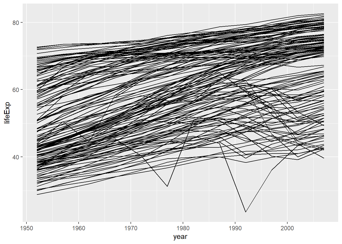
Overall, life expectancy has been steadily increasing over time, but we need some estimation of the trend in individual countries. A possible way to do this would be to fit a linear model to the data from each country and look at the estimate. Given the 142 countries in the dataset, we really do not want to run the code for each one manually with copy-pasted code. Because we want to work at the country level, we will now nest our data by country.
by_country <- gapminder_df |>
  nest(.by = country)
by_country
# A tibble: 142 × 2
country data
<chr> <list>
1 Afghanistan <tibble [12 × 5]>
2 Albania <tibble [12 × 5]>
3 Algeria <tibble [12 × 5]>
4 Angola <tibble [12 × 5]>
5 Argentina <tibble [12 × 5]>
6 Australia <tibble [12 × 5]>
7 Austria <tibble [12 × 5]>
8 Bahrain <tibble [12 × 5]>
9 Bangladesh <tibble [12 × 5]>
10 Belgium <tibble [12 × 5]>
# ℹ 132 more rowsIn the data column we now have a tibble with 12 rows and 5 columns for each country. We can access one of them, for example, Austria, using the [[]].
by_country$data[[7]]# A tibble: 12 × 5
year continent lifeExp pop gdpPercap
<dbl> <chr> <dbl> <dbl> <dbl>
1 1952 Europe 66.8 6927772 6137.
2 1957 Europe 67.5 6965860 8843.
3 1962 Europe 69.5 7129864 10751.
4 1967 Europe 70.1 7376998 12835.
5 1972 Europe 70.6 7544201 16662.
6 1977 Europe 72.2 7568430 19749.
7 1982 Europe 73.2 7574613 21597.
8 1987 Europe 74.9 7578903 23688.
9 1992 Europe 76.0 7914969 27042.
10 1997 Europe 77.5 8069876 29096.
11 2002 Europe 79.0 8148312 32418.
12 2007 Europe 79.8 8199783 36126.To calculate a linear model for data from each country, we will iterate over the data column and save the resulting model to a new column. This might be done with map() within the mutate() call.
by_country <- gapminder_df |>
  nest(.by = country) |>
  mutate(m = map(data, ~lm(lifeExp~year, data = .x)))
by_country
# A tibble: 142 × 3
country data m
<chr> <list> <list>
1 Afghanistan <tibble [12 × 5]> <lm>
2 Albania <tibble [12 × 5]> <lm>
3 Algeria <tibble [12 × 5]> <lm>
4 Angola <tibble [12 × 5]> <lm>
5 Argentina <tibble [12 × 5]> <lm>
6 Australia <tibble [12 × 5]> <lm>
7 Austria <tibble [12 × 5]> <lm>
8 Bahrain <tibble [12 × 5]> <lm>
9 Bangladesh <tibble [12 × 5]> <lm>
10 Belgium <tibble [12 × 5]> <lm>
# ℹ 132 more rowsThe column m we just created is again a list and contains the results of linear models for the relationship between life expectancy and time for all countries. With each one of them, we can do whatever is possible with a model result:
summary(by_country$m[[7]])
Call:
lm(formula = lifeExp ~ year, data = .x)

Residuals:
     Min       1Q   Median       3Q      Max
-0.65831 -0.21588  0.04173  0.21680  0.67162

Coefficients:
              Estimate Std. Error t value Pr(>|t|)
(Intercept) -4.059e+02  1.349e+01  -30.09 3.84e-11 ***
year         2.420e-01  6.814e-03   35.52 7.44e-12 ***
---
Signif. codes:  0 '***' 0.001 '**' 0.01 '*' 0.05 '.' 0.1 ' ' 1

Residual standard error: 0.4074 on 10 degrees of freedom
Multiple R-squared:  0.9921,    Adjusted R-squared:  0.9913
F-statistic:  1261 on 1 and 10 DF,  p-value: 7.435e-12
To easily extract the estimates from the model, we will use tidy() function from the broom package. broom is not part of the tidyverse, but it is a related package, which becomes very helpful when working with models within the tidyverse workflow, because it provides tools to convert statistical objects into tidy tibbles. The tidy() function summarises information about the model components:
tidy(by_country$m[[7]])# A tibble: 2 × 5
term estimate std.error statistic p.value
<chr> <dbl> <dbl> <dbl> <dbl>
1 (Intercept) -406. 13.5 -30.1 3.84e-11
2 year 0.242 0.00681 35.5 7.44e-12And we can again use it to iterate over all models to get these summaries for all countries.
by_country <- gapminder_df |>
  nest(.by = country) |>
  mutate(m = map(data, ~lm(lifeExp~year, data = .x)),
         m_tidy = map(m, ~tidy(.x)))

glimpse(by_country)
Rows: 142
Columns: 4
$ country <chr> "Afghanistan", "Albania", "Algeria", "Angola", "Argentina", "A…
$ data <list> [<tbl_df[12 x 5]>], [<tbl_df[12 x 5]>], [<tbl_df[12 x 5]>], […
$ m <list> [-507.5342716, 0.2753287, -1.10629487, -0.95193823, -0.663581…
$ m_tidy <list> [<tbl_df[2 x 5]>], [<tbl_df[2 x 5]>], [<tbl_df[2 x 5]>], [<tb…The summary is now in a tibble, but there is still a list of tibbles in the m_tidy column. To get the results to a data frame where we can sort the values and filter across all values, we need to unnest().
by_country <- gapminder_df |>
  nest(.by = country) |>
  mutate(m = map(data, ~lm(lifeExp~year, data = .x)),
         m_tidy = map(m, ~tidy(.x))) |>
  unnest(m_tidy)

glimpse(by_country)
Rows: 284
Columns: 8
$ country <chr> "Afghanistan", "Afghanistan", "Albania", "Albania", "Algeria…
$ data <list> [<tbl_df[12 x 5]>], [<tbl_df[12 x 5]>], [<tbl_df[12 x 5]>],…
$ m <list> [-507.5342716, 0.2753287, -1.10629487, -0.95193823, -0.6635…
$ term <chr> "(Intercept)", "year", "(Intercept)", "year", "(Intercept)",…
$ estimate <dbl> -507.5342716, 0.2753287, -594.0725110, 0.3346832, -1067.8590…
$ std.error <dbl> 40.484161954, 0.020450934, 65.655359062, 0.033166387, 43.802…
$ statistic <dbl> -12.536613, 13.462890, -9.048348, 10.091036, -24.379118, 25.…
$ p.value <dbl> 1.934055e-07, 9.835213e-08, 3.943337e-06, 1.462763e-06, 3.07…We now have one column for each column originally included in the tibbles inside m_tidy. The list-columns we did not unnest still remain list-columns. There are now two rows for each country, one for each model coefficient - the intercept and the year. We are not interested in model intercepts now, so we can filter them out. To see in which countries has the life expectancy risen the most over time, we can arrange the dataset according to the model estimate.
by_country <- gapminder_df |>
  nest(.by = country) |>
  mutate(m = map(data, ~lm(lifeExp~year, data = .x)),
         m_tidy = map(m, ~tidy(.x))) |>
  unnest(m_tidy) |>
  filter(term == 'year') |>
  arrange(desc(estimate))

glimpse(by_country)
Rows: 142
Columns: 8
$ country <chr> "Oman", "Vietnam", "Saudi Arabia", "Indonesia", "Libya", "Ye…
$ data <list> [<tbl_df[12 x 5]>], [<tbl_df[12 x 5]>], [<tbl_df[12 x 5]>],…
$ m <list> [-1470.085705, 0.772179, 0.3702564, -0.9886387, -1.7645338,…
$ term <chr> "year", "year", "year", "year", "year", "year", "year", "yea…
$ estimate <dbl> 0.7721790, 0.6716154, 0.6496231, 0.6346413, 0.6255357, 0.605…
$ std.error <dbl> 0.039265234, 0.021970572, 0.034812325, 0.010796685, 0.025754…
$ statistic <dbl> 19.665718, 30.568863, 18.660721, 58.781125, 24.288551, 22.82…
$ p.value <dbl> 2.530346e-09, 3.289412e-11, 4.221338e-09, 4.931386e-14, 3.18…Or we can just print out the top 10 countries:
by_country |> slice_max(estimate, n = 10)# A tibble: 10 × 8
country data m term estimate std.error statistic p.value
<chr> <list> <lis> <chr> <dbl> <dbl> <dbl> <dbl>
1 Oman <tibble> <lm> year 0.772 0.0393 19.7 2.53e- 9
2 Vietnam <tibble> <lm> year 0.672 0.0220 30.6 3.29e-11
3 Saudi Arabia <tibble> <lm> year 0.650 0.0348 18.7 4.22e- 9
4 Indonesia <tibble> <lm> year 0.635 0.0108 58.8 4.93e-14
5 Libya <tibble> <lm> year 0.626 0.0258 24.3 3.19e-10
6 Yemen, Rep. <tibble> <lm> year 0.605 0.0265 22.8 5.87e-10
7 West Bank and Gaza <tibble> <lm> year 0.601 0.0332 18.1 5.59e- 9
8 Tunisia <tibble> <lm> year 0.588 0.0261 22.5 6.64e-10
9 Gambia <tibble> <lm> year 0.582 0.0192 30.3 3.57e-11
10 Jordan <tibble> <lm> year 0.572 0.0319 17.9 6.31e- 9The use of nested data frames and broom has great potential. Depending on the question, it is possible to filter only significant results, select models with the highest explanatory power, etc. To learn more about the automatisation using purrr and running many models, look here: https://r4ds.hadley.nz/iteration.html, https://adv-r.hadley.nz/functionals.html, https://r4ds.had.co.nz/many-models.html, https://www.tmwr.org.
7.3.5 Debugging
It is possible that the code may not work initially. To simplify iteration within map(), it is often helpful to perform the calculation for a single element of the list and try to identify the error there. We can do this by replacing .x by one element of our nested tibble.
by_country <- gapminder_df |>
  nest(.by = country)

lm(lifeExp~year, data = by_country$data[[1]])
Call:
lm(formula = lifeExp ~ year, data = by_country$data[[1]])

Coefficients:
(Intercept)         year
  -507.5343       0.2753
7.4 Exercises
Rewrite the following code as a function:
x / sum(x, na.rm = T)*100
y / sum(y, na.rm = T)*100
z / sum(z, na.rm = T)*100
Use the function to calculate the percentage of each species in the penguins dataset.
Write your own function that takes a numeric vector of temperatures in Fahrenheit and returns them converted to Celsius using the formula \(C = (F-32) *5/9\). Test it with the following values: 0°F, 20°F, 68°F, 86°F, 100°F.
In Turboveg 2, a programme used for storing vegetation plot data, the geographical coordinates are stored in a format DDMMSS.SS. To show the plots in the map or perform any spatial calculations, you will need to transform the coordinates to decimal degrees. That is the purpose of the following function:
 tv_to_degrees <- function(coord){
  as.numeric(str_sub(coord, 1, 2)) + as.numeric(str_sub(coord, 3, 4)) / 60 + as.numeric(str_sub(coord, 5, 11)) / 3600
}
Look at the function and try to explain how it works. Load the basiphilous grassland data (
basiphilous_grasslands/basiphilous_grasslands_S_Moravia_head.csv, Link to the Github folder) and use this function to transform coordinates in the fieldsLongitudeandLatitude.Write a function that calculates the heat load index using measured values of slope and aspect in a vegetation plot. You will need the following formula (McCune & Keon, 2002):
\[ 0.339 + 0.808 \cdot \cos\left(\frac{\text{latitude} \cdot \pi}{180}\right) \cdot \cos\left(\frac{\text{slope} \cdot \pi}{180}\right)- 0.196 \cdot \sin\left(\frac{\text{latitude} \cdot \pi}{180}\right) \cdot \sin\left(\frac{\text{slope} \cdot \pi}{180}\right)- 0.482 \cdot \cos\left(\frac{\left|180 - \left|\text{aspect} - 225\right|\right| \cdot \pi}{180}\right) \cdot \sin\left(\frac{\text{slope} \cdot \pi}{180}\right) \]
0.339+0.808*cos(DEG_LAT*pi/180)*cos(SLOPE*pi/180)-0.196*sin(DEG_LAT*pi/180)*sin(SLOPE*pi/180)-0.482*cos((abs(180-abs(ASPECT-225)))*pi/180)*sin(SLOPE*pi/180)
Use the function to calculate the heat load index for vegetation plots in basiphilous grasslands (use the same data as in the previous exercise). * Calculate species richness of the plots and plot the relationship between the heat load index and species richness. Select only plots sampled in 2022 which are more precisely located. (Use the species data
basiphilous_grasslands/basiphilous_grasslands_S_Moravia_species.csv, transform them to the long format, calculate the number of species per plot and join this information to the header data before you start plotting).Write a function to calculate the logistic population growth using the formula \(N_t = \frac{K}{1 + \left( \frac{K - N_0}{N_0} \right) e^{-r t}}\), where \(N_0\) is the initial population, K the carrying capacity, r an intrinsic growth rate and t time. Run the function for the values \(N_0 = 10\), K = 100, r = 0.3 and time varies from 1 to 20.
K / (1 + ((K - N0) / N0) * exp(-r * t))
* Write a function that calculates the Shannon diversity index using the formula \(H' = -∑p_i ln(p_i)\). Use the function to calculate Shannon diversity of each plot in the sand vegetation dataset.
Take the Pokémon dataset (
read_csv('https://raw.githubusercontent.com/rfordatascience/tidytuesday/main/data/2025/2025-04-01/pokemon_df.csv')) and visualise the distribution of defense power of water-type Pokémon. Turn this code into a function that helps you draw a histogram of defense power for different Pokémon types. * Try to generalize the code so that you can plot a distribution of any numerical variable.Use the function in a for loop and create plots of the distribution of defense power for all Pokémon types. * Save all plots in a
plotsfolder.Use a function from the
purrrpackage to calculate the logaritm of each value in the following list:test_list <- list(0, 1, 4, 8, 10). Save the output first as a list and second as a numeric vector. Compare the differences.Take the following numeric vectors and use a function from the
purrrpackage to multiply the first one by the second one.num1 <- list(1, 2, 3, 4, 5, 6),num2 <- list(7, 8, 9, 10, 11, 12). Save the output first as a list and second as a numeric vector. Compare the differences.Use the function from exercise 9 and create plots of the distribution of defense power for all Pokémon types using functions from the
purrrpackage.In this exercise, we will use data of the 10 most common frog species recorded within the Australian FrogID initiative. The original data comes from the TidyTuesdays repository, but we modified it slightly for this exercise and stored it in the
frogsfolder of our repository. The data are stored in multiple csv files, one for each species. Load all these files using a single pipeline and save to your environment as a single tibble. Store the species names in a column in the final tibble.* Create a bar plot showing which frog species are most often recorded (to order the species from the most to the least common, use a function from the
forcats()package). Add colour distinction of records from different territories (columnstateProvince).Save the frog data as separate csv files by territory, where the observations were made in a folder
frogs_territory.* Use the Pokémon dataset, nest it by Pokémon type and calculate linear models for the relationship between defense and attack power (
lm(defense ~ attack)) of each Pokémon type using amap()function withinmutate(). Use thetidy()function to extract coefficients and p-values from the model. Unnest the list column where you saved the results oftidy(). For each Pokémon type, filter only statistics for the attack coefficient, keep only significant results (p < 0.05) and arrange the dataset according to the coefficient from the linear model from Pokémon types where the relationship between defence and attack power is the strongest to those with the weakest relationship.* Take the code for visualisation of Ellenberg-type indicator values in different forest types (Exercise 5 in Chapter 6) and turn it into a function. Draw the boxplots for four different Ellenberg-type indicator values using this function. Use a for loop or
purrrfunctions to make these four plots. Combine them and save them in theplotsfolder.
7.5 Further reading
R for Data Science: https://r4ds.hadley.nz/program.html
Hands on Programming with R: https://rstudio-education.github.io/hopr
Advanced R: https://adv-r.hadley.nz
Tidy Modeling with R: https://www.tmwr.org
Programming with dplyr: https://dplyr.tidyverse.org/articles/programming.html
Programming with tidyr: https://tidyr.tidyverse.org/articles/programming.html
Programming with ggplot2: https://ggplot2-book.org/programming.html
Tidy modeling with R: https://www.tmwr.org
References
McCune, B., & Keon, D. (2002). Equations for potential annual direct incident radiation and heat load. Journal of Vegetation Science, 13(4), 603–606. https://doi.org/10.1111/j.1654-1103.2002.tb02087.x