library(tidyverse)
library(readxl)
library(janitor) 11 From a database to a plot
This tutorial aims to repeat what we have learned so far. We will step by step show you how to import data from a database into R, prepare it for further analysis, and provide some basic summaries of the data, as well as plot answers to our questions. At the end of this chapter, you will find the final exercises that we would like you to complete and hand in. The script will then be considered your final project for this course.
11.1 Example of database format data / Turboveg
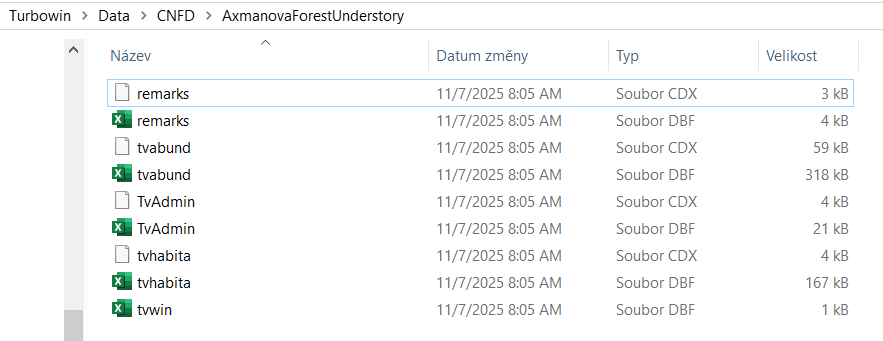
Turboveg for Windows is a program designed for storing, selecting, and exporting vegetation plot data (relevés). The information is divided among several files that are matched by either species ID or releve ID. Within the Turboveg interface, you do not see this structure directly; however, you can find it by looking in the Turbowin folder, subfolder Data, and a particular database (see example below).
At some point, you need to export the data and process it further. To get Turboveg data to R, you first need to export the Turboveg database to a folder where you want to process the data. This step requires the selection of all the plots you want to export. Alternatively, you can access the files directly in the main file in Turbowin. However, please note that if you make an error here, you may lose your data altogether.
11.2 Load libraries
11.3 Import env file = headers
One option is to manually check the exported database by opening the file called tvhabita.dbf in Excel and saving it as a tvhabita.xlsx or tvhabita.csv (UTF-8 encoded) file in your data folder. Although it involves one additional step outside R, it remains relatively straightforward and saves you trouble with different formats in Turboveg and R (encoding issues). Another option is to open the dbf files directly, for example, with the foreign package.
You can then import the file as csv file.
env <- read_csv("data/turboveg_to_R/tvhabita.csv")Rows: 137 Columns: 84
── Column specification ────────────────────────────────────────────────────────
Delimiter: ","
chr (13): COUNTRY, COVERSCALE, AUTHOR, SYNTAXON, MOSS_IDENT, LICH_IDENT, REM...
dbl (45): RELEVE_NR, DATE, SURF_AREA, ALTITUDE, EXPOSITION, INCLINATIO, COV_...
lgl (26): REFERENCE, TABLE_NR, NR_IN_TAB, PROJECT, UTM, RESURVEY, FOR_EVA, R...
ℹ Use `spec()` to retrieve the full column specification for this data.
ℹ Specify the column types or set `show_col_types = FALSE` to quiet this message.If you check the imported names, you will find that they are somewhat challenging to handle.
names(env) [1] "RELEVE_NR" "COUNTRY" "REFERENCE" "TABLE_NR" "NR_IN_TAB"
[6] "COVERSCALE" "PROJECT" "AUTHOR" "DATE" "SYNTAXON"
[11] "SURF_AREA" "UTM" "ALTITUDE" "EXPOSITION" "INCLINATIO"
[16] "COV_TOTAL" "COV_TREES" "COV_SHRUBS" "COV_HERBS" "COV_MOSSES"
[21] "COV_LICHEN" "COV_ALGAE" "COV_LITTER" "COV_WATER" "COV_ROCK"
[26] "TREE_HIGH" "TREE_LOW" "SHRUB_HIGH" "SHRUB_LOW" "HERB_HIGH"
[31] "HERB_LOW" "HERB_MAX" "CRYPT_HIGH" "MOSS_IDENT" "LICH_IDENT"
[36] "REMARKS" "COORD_CODE" "SYNTAX_OLD" "RESURVEY" "FOR_EVA"
[41] "RS_PROJECT" "RS_SITE" "RS_PLOT" "RS_OBSERV" "PLOT_SHAPE"
[46] "MANIPULATE" "MANIPTYP" "LOC_METHOD" "DATA_OWNER" "EVA_ACCESS"
[51] "LONGITUDE" "LATITUDE" "PRECISION" "LOCALITY" "BIAS_MIN"
[56] "BIAS_GPS" "CEBA_GRID" "FIELD_NR" "HABITAT" "GEOLOGY"
[61] "SOIL" "WATER_PH" "S_PH_H2O" "S_PH_KCL" "S_PH_CACL2"
[66] "SOIL_PH" "CONDUCT" "NR_ORIG" "HLOUBK_CM" "DNO"
[71] "CEL_PLO_M2" "ZAROST_PLO" "ESY_CODE" "ESY_NAME" "COV_WOOD"
[76] "SOIL_DPT" "TRAMPLING" "PLOT_TYPE" "RS_CODE" "RS_PROJTYP"
[81] "RADIATION" "HEAT" "LES" "NELES" Therefore, we will directly change them to tidy names using the clean_names() function from the janitor package. An alternative is to rename one by one using e.g. rename(), but here we want to save time and effort.
env <- read_csv("data/turboveg_to_R/tvhabita.csv") %>%
  clean_names()
Rows: 137 Columns: 84
── Column specification ────────────────────────────────────────────────────────
Delimiter: ","
chr (13): COUNTRY, COVERSCALE, AUTHOR, SYNTAXON, MOSS_IDENT, LICH_IDENT, REM...
dbl (45): RELEVE_NR, DATE, SURF_AREA, ALTITUDE, EXPOSITION, INCLINATIO, COV_...
lgl (26): REFERENCE, TABLE_NR, NR_IN_TAB, PROJECT, UTM, RESURVEY, FOR_EVA, R...
ℹ Use `spec()` to retrieve the full column specification for this data.
ℹ Specify the column types or set `show_col_types = FALSE` to quiet this message.tibble(env)# A tibble: 137 × 84
releve_nr country reference table_nr nr_in_tab coverscale project author
<dbl> <chr> <lgl> <lgl> <lgl> <chr> <lgl> <chr>
1 183111 CZ NA NA NA 02 NA 0832
2 183112 CZ NA NA NA 02 NA 0832
3 183113 CZ NA NA NA 02 NA 0832
4 183114 CZ NA NA NA 02 NA 0832
5 183115 CZ NA NA NA 02 NA 0832
6 183116 CZ NA NA NA 02 NA 0832
7 183117 CZ NA NA NA 02 NA 0832
8 183118 CZ NA NA NA 02 NA 0832
9 183119 CZ NA NA NA 02 NA 0832
10 183120 CZ NA NA NA 02 NA 0832
# ℹ 127 more rows
# ℹ 76 more variables: date <dbl>, syntaxon <chr>, surf_area <dbl>, utm <lgl>,
# altitude <dbl>, exposition <dbl>, inclinatio <dbl>, cov_total <dbl>,
# cov_trees <dbl>, cov_shrubs <dbl>, cov_herbs <dbl>, cov_mosses <dbl>,
# cov_lichen <dbl>, cov_algae <dbl>, cov_litter <dbl>, cov_water <dbl>,
# cov_rock <dbl>, tree_high <dbl>, tree_low <dbl>, shrub_high <dbl>,
# shrub_low <dbl>, herb_high <dbl>, herb_low <dbl>, herb_max <dbl>, …names(env) [1] "releve_nr" "country" "reference" "table_nr" "nr_in_tab"
[6] "coverscale" "project" "author" "date" "syntaxon"
[11] "surf_area" "utm" "altitude" "exposition" "inclinatio"
[16] "cov_total" "cov_trees" "cov_shrubs" "cov_herbs" "cov_mosses"
[21] "cov_lichen" "cov_algae" "cov_litter" "cov_water" "cov_rock"
[26] "tree_high" "tree_low" "shrub_high" "shrub_low" "herb_high"
[31] "herb_low" "herb_max" "crypt_high" "moss_ident" "lich_ident"
[36] "remarks" "coord_code" "syntax_old" "resurvey" "for_eva"
[41] "rs_project" "rs_site" "rs_plot" "rs_observ" "plot_shape"
[46] "manipulate" "maniptyp" "loc_method" "data_owner" "eva_access"
[51] "longitude" "latitude" "precision" "locality" "bias_min"
[56] "bias_gps" "ceba_grid" "field_nr" "habitat" "geology"
[61] "soil" "water_ph" "s_ph_h2o" "s_ph_kcl" "s_ph_cacl2"
[66] "soil_ph" "conduct" "nr_orig" "hloubk_cm" "dno"
[71] "cel_plo_m2" "zarost_plo" "esy_code" "esy_name" "cov_wood"
[76] "soil_dpt" "trampling" "plot_type" "rs_code" "rs_projtyp"
[81] "radiation" "heat" "les" "neles" We will prepare a selection of the variables we want to keep and rewrite the file. Always keep releve_nr and coverscale, as you will need them later on.
env <- env %>%
  select(releve_nr, coverscale,field_nr, country, author, date, syntaxon,
         altitude, exposition, inclinatio,
         cov_trees, cov_shrubs, cov_herbs, cov_mosses,
         latitude, longitude, precision, bias_min, bias_gps, locality)
Alternatively, we can combine all the steps we’ve taken so far into a single pipeline and check the resulting dataset.
env <- read_csv("data/turboveg_to_R/tvhabita.csv") %>%
  clean_names() %>%
  select(releve_nr, coverscale, field_nr, country, author, date, syntaxon,
         altitude, exposition, inclinatio,
         cov_trees, cov_shrubs, cov_herbs, cov_mosses,
         latitude, longitude, precision, bias_min, bias_gps, locality) %>%
  glimpse()
Rows: 137 Columns: 84
── Column specification ────────────────────────────────────────────────────────
Delimiter: ","
chr (13): COUNTRY, COVERSCALE, AUTHOR, SYNTAXON, MOSS_IDENT, LICH_IDENT, REM...
dbl (45): RELEVE_NR, DATE, SURF_AREA, ALTITUDE, EXPOSITION, INCLINATIO, COV_...
lgl (26): REFERENCE, TABLE_NR, NR_IN_TAB, PROJECT, UTM, RESURVEY, FOR_EVA, R...
ℹ Use `spec()` to retrieve the full column specification for this data.
ℹ Specify the column types or set `show_col_types = FALSE` to quiet this message.Rows: 137
Columns: 20
$ releve_nr <dbl> 183111, 183112, 183113, 183114, 183115, 183116, 183117, 183…
$ coverscale <chr> "02", "02", "02", "02", "02", "02", "02", "02", "02", "02",…
$ field_nr <chr> "2/2007", "3/2007", "4/2007", "5/2007", "6/2007", "7/2007",…
$ country <chr> "CZ", "CZ", "CZ", "CZ", "CZ", "CZ", "CZ", "CZ", "CZ", "CZ",…
$ author <chr> "0832", "0832", "0832", "0832", "0832", "0832", "0832", "08…
$ date <dbl> 20070702, 20070702, 20070702, 20070703, 20070703, 20070703,…
$ syntaxon <chr> "LDA01", "LDA01", "LDA", "LDA01", "LDA", "LD", "LBB", "LB",…
$ altitude <dbl> 458, 414, 379, 374, 380, 373, 390, 255, 340, 368, 356, 427,…
$ exposition <dbl> 150, 150, 210, NA, 170, 65, NA, 80, 220, 95, 200, 170, 130,…
$ inclinatio <dbl> 24, 13, 21, 0, 10, 6, 0, 38, 13, 29, 38, 27, 7, 22, 9, 21, …
$ cov_trees <dbl> 80, 80, 75, 70, 65, 65, 85, 80, 70, 85, 45, 70, 65, 70, 80,…
$ cov_shrubs <dbl> 0, 0, 0, 0, 1, 0, 0, 20, 0, 15, 1, 0, 2, 1, 12, 0, 0, 0, 0,…
$ cov_herbs <dbl> 25, 25, 30, 35, 60, 70, 70, 15, 75, 8, 75, 40, 60, 40, 60, …
$ cov_mosses <dbl> 10, 8, 10, 8, 3, 5, 5, 10, 3, 5, 20, 3, 5, 30, 1, 5, 1, 5, …
$ latitude <dbl> 492015.3, 492128.9, 492126.4, 490210.2, 490203.1, 490158.5,…
$ longitude <dbl> 163420.0, 163345.8, 162913.4, 162137.8, 162128.3, 162117.2,…
$ precision <dbl> 0, 0, 0, 0, 0, 0, 0, 0, 0, 0, 0, 0, 0, 0, 0, 0, 0, 0, 0, 0,…
$ bias_min <dbl> 0, 0, 0, 0, 0, 0, 0, 0, 0, 0, 0, 0, 0, 0, 0, 0, 0, 0, 0, 0,…
$ bias_gps <dbl> 5, 6, 10, 6, 5, 6, 14, 6, 4, 5, 5, 5, 6, 6, 5, 11, 8, 7, 4,…
$ locality <chr> "Svinošice (Brno, Kuřim); 450 m SZ od středu obce", "Lažany…And save it for easier access.
write.csv(env, "data/turboveg_to_R/env.csv")11.4 Import spe file = species file in a long format
Again, we will open the tvabund.dbf in Excel and save it as tvabund.csv. And import it to our environment in R. Again, we will use the clean_names() function during import, so that we have the same style of variable names.
tvabund <- read_csv("data/turboveg_to_R/tvabund.csv") %>%
  clean_names()
Rows: 4583 Columns: 5
── Column specification ────────────────────────────────────────────────────────
Delimiter: ","
chr (1): COVER_CODE
dbl (3): RELEVE_NR, SPECIES_NR, LAYER
lgl (1): _ORIG_NAME
ℹ Use `spec()` to retrieve the full column specification for this data.
ℹ Specify the column types or set `show_col_types = FALSE` to quiet this message.glimpse(tvabund)Rows: 4,583
Columns: 5
$ releve_nr <dbl> 183111, 183111, 183111, 183111, 183111, 183111, 183111, 183…
$ species_nr <dbl> 2206, 2315, 3351, 4283, 4430, 4577, 5127, 5137, 5165, 5353,…
$ cover_code <chr> "+", "1", "r", "1", "r", "r", "1", "+", "r", "r", "2b", "+"…
$ layer <dbl> 6, 7, 6, 6, 7, 6, 6, 6, 6, 6, 6, 6, 6, 6, 1, 7, 6, 6, 6, 6,…
$ orig_name <lgl> NA, NA, NA, NA, NA, NA, NA, NA, NA, NA, NA, NA, NA, NA, NA,…Now we will check the data again, and we see that there are no species names, just numbers. Additionally, the cover is provided in the original codes, not in percentages. Refer to the scheme below to understand where each piece of information is stored.
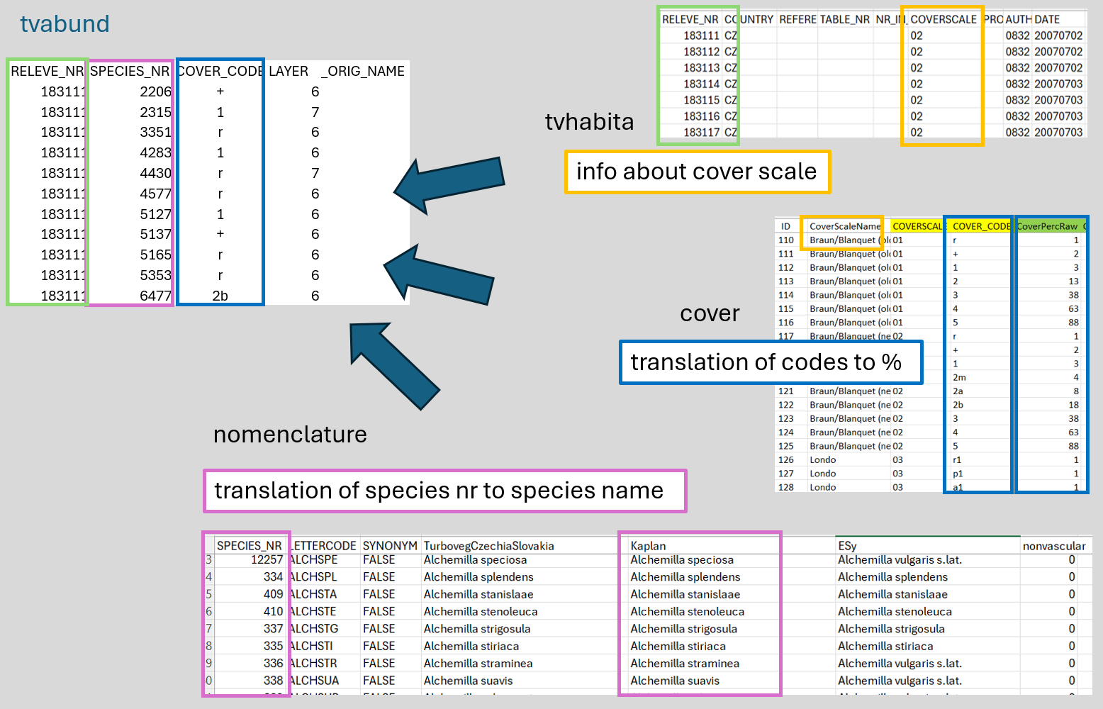
We need to prepare the different files, import them, and merge them.
11.4.1 Nomenclature
In the abund file, species numbers refer to the codes in the checklist used in the Turboveg database. To translate them into species names, you will need a translation table with the original number in the database, the original name in the database and the name you want to use in the analyses.
We will now import the nomenclature file, which is already adapted for the Czech flora.
nomenclature <- read_csv("data/turboveg_to_R/nomenclature_20251108.csv") %>%
  clean_names()
Rows: 13862 Columns: 7
── Column specification ────────────────────────────────────────────────────────
Delimiter: ","
chr (4): LETTERCODE, TurbovegCzechiaSlovakia, Kaplan, ExpertSystem
dbl (2): SPECIES_NR, nonvascular
lgl (1): SYNONYM
ℹ Use `spec()` to retrieve the full column specification for this data.
ℹ Specify the column types or set `show_col_types = FALSE` to quiet this message.tibble(nomenclature)# A tibble: 13,862 × 7
species_nr lettercode synonym turboveg_czechia_slovakia kaplan expert_system
<dbl> <chr> <lgl> <chr> <chr> <chr>
1 14321 *CONC*C FALSE x Conygeron huelsenii x Con… x Conyzigero…
2 14323 *DACD*A FALSE x Dactylodenia gracilis x Dac… x Dactylogym…
3 14324 *DACD*A TRUE x Dactylodenia st.-quinti… x Dac… x Dactylogym…
4 14322 *DACD*D FALSE x Dactylodenia comigera x Dac… x Dactylogym…
5 14325 *DATD*D FALSE x Dactyloglossum erdingeri x Dac… x Dactyloglo…
6 14327 *FESF*E FALSE x Festulolium loliaceum x Fes… x Festuloliu…
7 14326 *FESF*F FALSE x Festulolium braunii x Fes… x Festuloliu…
8 14328 *GYMG*G FALSE x Gymnanacamptis anacampt… x Gym… x Gymnanacam…
9 14329 *ORCO*O FALSE x Orchidactyla boudieri x Dac… x Dactylocam…
10 14330 *PSEP*P FALSE x Pseudadenia schweinfurt… x Pse… x Pseudadeni…
# ℹ 13,852 more rows
# ℹ 1 more variable: nonvascular <dbl>There are several advantages to this approach. First, you can adjust the nomenclature to the newest source/regional checklist, etc. In our example, the name in Turboveg is translated to the nomenclature presented in the recent Key of the Czech Flora, and it is named after the main editor, Kaplan.
Second, I can add a concept that groups several taxa into higher units, e.g., taxa that are not easily recognisable in the field are assigned to aggregates. This is the same approach you use when creating an expert system file. Here, it is even easier to understand and much easier to change the translation when you need to make a correction. The name in this file is called ESy.
Last but not least. We can directly add much more information to such a table, for example, status, growth form or anything else. Here, we indicate whether the species is nonvascular.
We might want to check how the species are translated using my translation file and select only these matching rows. Either create a variable called ‘selection’ to indicate whether the species is in the subset or not.
nomenclature_check <- nomenclature %>%
  left_join(tvabund %>%
              distinct(species_nr) %>%
              mutate(selection = 1))
Joining with `by = join_by(species_nr)`Alternatively, we can also add the frequency, which indicates how many times it appears in the dataset’s records.
nomenclature_check <- nomenclature %>%
  left_join(tvabund %>%
              count(species_nr))
Joining with `by = join_by(species_nr)`We can then write the file, make adjustments (e.g., in Excel), and upload it again. The great thing is that we have an indication of which species are in the dataset, and we do not have to pay attention to the other rows.
write.csv(nomenclature_check, "data/turboveg_to_R/nomenclature_check.csv")Upload the new, adjusted file:
nomenclature <- read_csv("data/turboveg_to_R/nomenclature_check.csv") %>%
  clean_names()
11.4.2 Cover
We have a translation table for nomenclature, but we still need to translate cover codes to percentages. For cover translation, we need to use information about the cover scale (stored in the header data / tvhabita / env file) and information on how to translate the values in that particular scale to percentages. The file here was prepared based on translating cover values in different scales to percentages, following the EVA database approach. One more column was added to enable different adjustments, such as changing the values for rare species, etc. For any project, I suggest opening the file and verifying that the scales you are using are present and that you agree with the translation.
cover <- read_csv("data/turboveg_to_R/cover_20230402.csv") %>%
  clean_names()
Rows: 326 Columns: 6
── Column specification ────────────────────────────────────────────────────────
Delimiter: ","
chr (3): CoverScaleName, COVERSCALE, COVER_CODE
dbl (3): ID, CoverPercEVA, CoverPerc
ℹ Use `spec()` to retrieve the full column specification for this data.
ℹ Specify the column types or set `show_col_types = FALSE` to quiet this message.tibble(cover)# A tibble: 326 × 6
id cover_scale_name coverscale cover_code cover_perc_eva cover_perc
<dbl> <chr> <chr> <chr> <dbl> <dbl>
1 1 Percetage % 00 0.1 0.1 0.1
2 2 Percetage % 00 0.2 0.2 0.2
3 3 Percetage % 00 0.3 0.3 0.3
4 4 Percetage % 00 0.4 0.4 0.4
5 5 Percetage % 00 0.5 0.5 0.5
6 6 Percetage % 00 0.6 0.6 0.6
7 7 Percetage % 00 0.7 0.7 0.7
8 8 Percetage % 00 0.8 0.8 0.8
9 9 Percetage % 00 0.9 0.9 0.9
10 10 Percetage % 00 1 1 1
# ℹ 316 more rowsHere, we can check the different scale names included in the file:
cover %>% distinct(cover_scale_name) # A tibble: 16 × 1
cover_scale_name
<chr>
1 Percetage %
2 Braun/Blanquet (old)
3 Braun/Blanquet (new)
4 Londo
5 Presence/Absence
6 Ordinale scale (1-9)
7 Barkman, Doing & Segal
8 Doing
9 Domin
10 Sedlakova
11 Zlatnˇk
12 Percentual scale
13 Hedl
14 Kuźera
15 Domin (uprava Hadac)
16 Percentual (r, +) And we can also filter the rows of the specified scales. For example, here we are looking for all those that start with a specific pattern, “Braun”.
cover %>%
  filter(str_starts(cover_scale_name, "Braun")) %>%
  print(n = 20)
# A tibble: 16 × 6
id cover_scale_name coverscale cover_code cover_perc_eva cover_perc
<dbl> <chr> <chr> <chr> <dbl> <dbl>
1 110 Braun/Blanquet (old) 01 r 1 1
2 111 Braun/Blanquet (old) 01 + 2 2
3 112 Braun/Blanquet (old) 01 1 3 3
4 113 Braun/Blanquet (old) 01 2 13 13
5 114 Braun/Blanquet (old) 01 3 38 38
6 115 Braun/Blanquet (old) 01 4 63 63
7 116 Braun/Blanquet (old) 01 5 88 88
8 117 Braun/Blanquet (new) 02 r 1 0.1
9 118 Braun/Blanquet (new) 02 + 2 0.5
10 119 Braun/Blanquet (new) 02 1 3 3
11 120 Braun/Blanquet (new) 02 2m 4 4
12 121 Braun/Blanquet (new) 02 2a 8 10
13 122 Braun/Blanquet (new) 02 2b 18 20
14 123 Braun/Blanquet (new) 02 3 38 37.5
15 124 Braun/Blanquet (new) 02 4 63 62.5
16 125 Braun/Blanquet (new) 02 5 88 87.511.4.3 Merging all files into a complete spe file
Finally, we have both the translation to nomenclature and the translation to cover. Now we need to put everything together.
tvabund %>%
  left_join(nomenclature %>%
              select(species_nr, kaplan, expert_system, nonvascular)) %>%
  left_join(env %>% select(releve_nr, coverscale)) %>%
  left_join(cover %>% select(coverscale,cover_code,cover_perc))
Joining with `by = join_by(species_nr)`
Joining with `by = join_by(releve_nr)`
Joining with `by = join_by(cover_code, coverscale)`# A tibble: 4,583 × 10
releve_nr species_nr cover_code layer orig_name kaplan expert_system
<dbl> <dbl> <chr> <dbl> <lgl> <chr> <chr>
1 183111 2206 + 6 NA Carex digitata… Carex digita…
2 183111 2315 1 7 NA Carpinus betul… Carpinus bet…
3 183111 3351 r 6 NA Cytisus nigric… Cytisus nigr…
4 183111 4283 1 6 NA Festuca ovina Festuca ovina
5 183111 4430 r 7 NA Fraxinus excel… Fraxinus exc…
6 183111 4577 r 6 NA Galium rotundi… Galium rotun…
7 183111 5127 1 6 NA Hieracium lach… Hieracium la…
8 183111 5137 + 6 NA Hieracium muro… Hieracium mu…
9 183111 5165 r 6 NA Hieracium saba… Hieracium sa…
10 183111 5353 r 6 NA Hypericum perf… Hypericum pe…
# ℹ 4,573 more rows
# ℹ 3 more variables: nonvascular <dbl>, coverscale <chr>, cover_perc <dbl>The output contains these variables.
"releve_nr" "species_nr" "cover_code" "layer" "orig_name" "kaplan" "expert_system" "nonvascular" "coverscale" "cover_perc" If we are satisfied with the result, we assign the pipeline to the spe file. We still want to add one more line to remove non-vascular plants (mosses) and add another line to select only the necessary variables. We decided to follow the concept saved in the expert_systemname, and renamed it directly in the select function.
spe <- tvabund %>%
  left_join(nomenclature %>%
              select(species_nr, kaplan, expert_system, nonvascular)) %>%
  left_join(env %>% select(releve_nr, coverscale)) %>%
  left_join(cover %>% select(coverscale, cover_code, cover_perc)) %>%
  filter(!nonvascular == 1) %>%
  select(releve_nr, species = expert_system, layer, cover_perc)
Joining with `by = join_by(species_nr)`
Joining with `by = join_by(releve_nr)`
Joining with `by = join_by(cover_code, coverscale)`To see the result, we will use view():
view(spe)We can again save the final file, to be easily accessible for later:
write.csv(spe, "data/turboveg_to_R/spe.csv")11.5 Merging of species covers
11.5.1 Duplicate species records
What is the problem? Sometimes we have some species names listed more than once in the same plot. Either because we changed the original concept (from subspecies to species level, or after additional identification) or because we recorded the same species in different layers. Depending on our further questions and analyses, this may become a minor or a more significant problem.
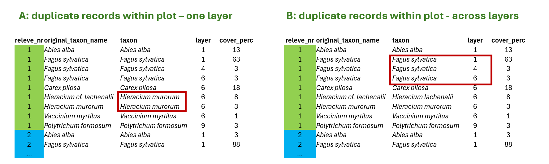
A) In the first case, duplicate within one layer, we can fix the problem by summing the values for the same species in the same layer to get distinct species-layer combinations per plot. This is something we need to do. Otherwise, our data would contradict the tidy approach, and we would encounter issues with joins, summarisation, etc.
B) In the other case, duplicate across layers, the data are OK, because there is one more variable that makes it a unique record (layer). However, if we want to examine the entire community, for example, calculating the share of certain life forms weighted by coverage, we again need to sum the values across layers and place all the species in the same layer (this is then typically marked as 0).
11.5.2 Duplicates checking
We recommend always performing the following data check. Simply group species by releves/plots and count if some of the species are in more rows.
spe %>%
  group_by(releve_nr, species, layer) %>%
  count() %>%
  filter(n > 1)
# A tibble: 2 × 4
# Groups: releve_nr, species, layer [2]
releve_nr species layer n
<dbl> <chr> <dbl> <int>
1 132 Galium palustre agg. 6 2
2 183182 Galium palustre agg. 6 2We can see that in two releves/plots, there is a conflict in the species Galium palustre agg. Most likely, we distinguished two species in the field that we later grouped into this aggregate. We can go back and check where exactly this happened by specifying where to look.
tvabund %>%
  select(releve_nr, species_nr)%>%
  left_join(nomenclature %>%
              select(species_nr, turboveg = turboveg_czechia_slovakia,
                     species = expert_system)) %>%
  filter(releve_nr %in% c(132, 183182) & species == "Galium palustre agg.")
Joining with `by = join_by(species_nr)`# A tibble: 4 × 4
releve_nr species_nr turboveg species
<dbl> <dbl> <chr> <chr>
1 183182 4558 Galium elongatum Galium palustre agg.
2 183182 4570 Galium palustre Galium palustre agg.
3 132 4558 Galium elongatum Galium palustre agg.
4 132 4570 Galium palustre Galium palustre agg.Alternatively, we can save the first output and use the semi_join() function, which is particularly useful when there are more rows to check, and we do not need to specify multiple conditions in the filter.
test <- spe %>%
  group_by(releve_nr, species, layer) %>%
  count() %>%
  filter(n > 1)


tvabund %>%
  select(releve_nr, species_nr) %>%
  left_join(nomenclature %>%
              select(species_nr, turboveg = turboveg_czechia_slovakia,
                     species = expert_system)) %>%
  semi_join(test)
Joining with `by = join_by(species_nr)`
Joining with `by = join_by(releve_nr, species)`# A tibble: 4 × 4
releve_nr species_nr turboveg species
<dbl> <dbl> <chr> <chr>
1 183182 4558 Galium elongatum Galium palustre agg.
2 183182 4570 Galium palustre Galium palustre agg.
3 132 4558 Galium elongatum Galium palustre agg.
4 132 4570 Galium palustre Galium palustre agg.Now that we understand why it happened, we need to address the issue. But we continue checking. Now we will check if there is also a problem with species across layers (B). We will simply change the grouping conditions to the higher hierarchy.
spe %>%
  group_by(releve_nr, species) %>%
  count() %>%
  filter(n > 1)
# A tibble: 375 × 3
# Groups: releve_nr, species [375]
releve_nr species n
<dbl> <chr> <int>
1 1 Acer campestre 2
2 1 Quercus petraea agg. 2
3 2 Quercus petraea agg. 2
4 3 Quercus petraea agg. 2
5 4 Carpinus betulus 2
6 4 Quercus petraea agg. 2
7 5 Quercus petraea agg. 2
8 6 Ligustrum vulgare 2
9 6 Quercus petraea agg. 2
10 6 Rosa species 2
# ℹ 365 more rowsWe got a lot of duplicates, right? However, it is understandable given the type of vegetation we have. Keep this in mind for later analyses.
Sometimes, it is actually good to take some extra time and look inside. Are only trees recorded, including shrubs and juveniles, or are some herbs mistakenly included in the tree layer? Use view() to see the whole list.
spe %>%
  distinct(species, layer) %>%
  group_by(species) %>%
  count() %>%
  filter(n > 1)
# A tibble: 38 × 2
# Groups: species [38]
species n
<chr> <int>
1 Acer campestre 3
2 Acer platanoides 3
3 Acer pseudoplatanus 3
4 Aesculus hippocastanum 2
5 Alnus glutinosa 3
6 Alnus incana 3
7 Carpinus betulus 3
8 Cornus mas 2
9 Cornus sanguinea 2
10 Corylus avellana 3
# ℹ 28 more rows11.5.3 Fixing duplicate rows
Now, finally, the fixing. For some questions, the easiest way to resolve duplicate rows is to select only the relevant variables and groups and use the distinct() function. For example, for species richness, this would be sufficient. BUT, we would lose information about the abundance, in our case, the percentage cover of each species.
spe %>%
  distinct(releve_nr, species, layer)
# A tibble: 4,575 × 3
releve_nr species layer
<dbl> <chr> <dbl>
1 183111 Carex digitata 6
2 183111 Carpinus betulus 7
3 183111 Cytisus nigricans 6
4 183111 Festuca ovina 6
5 183111 Fraxinus excelsior 7
6 183111 Galium rotundifolium 6
7 183111 Hieracium lachenalii 6
8 183111 Hieracium murorum 6
9 183111 Hieracium sabaudum s.lat. 6
10 183111 Hypericum perforatum 6
# ℹ 4,565 more rowsThe percentage cover is estimated visually relative to the total area. In the field, it is estimated independently of other plants, because we know that the plants overlap within vertical space. If we use the normal sum() function, we can easily get the total cover per plot above 100%. Although we can separate the information into vegetation layers, it remains a relatively coarse division, especially in grasslands, where the main diversity is concentrated in just one, often very dense, layer.
Therefore, we will use the approach suggested by H.S. Fischer in the paper On combination of species from different vegetation layers (AVS 2014), where he suggested summing up covers considering overlap among species, so that the overall maximum value is 100 and all the values are adjusted relative to this threshold. We will prepare a function called combine_cover().
combine_cover <- function(x){
  while (length(x)>1){
    x[2] <- x[1]+(100-x[1])*x[2]/100
    x <- x[-1]
  }
  return(x)
}
A) Now let’s check how it works. We will first fix the issue with duplicates within the same layer (A)
spe %>%
  group_by(releve_nr, species, layer) %>%
  summarise(cover_perc_new = combine_cover(cover_perc))
`summarise()` has grouped output by 'releve_nr', 'species'. You can override
using the `.groups` argument.# A tibble: 4,575 × 4
# Groups: releve_nr, species [4,138]
releve_nr species layer cover_perc_new
<dbl> <chr> <dbl> <dbl>
1 1 Acer campestre 1 20
2 1 Acer campestre 7 0.5
3 1 Acer platanoides 7 0.1
4 1 Anemone species 6 0.5
5 1 Bromus benekenii 6 0.1
6 1 Carex digitata 6 3
7 1 Carex michelii 6 0.1
8 1 Carex montana 6 0.5
9 1 Carpinus betulus 7 0.5
10 1 Cephalanthera damasonium 6 0.1
# ℹ 4,565 more rowsWe will also add pipelines to check for any remaining duplicate rows. Note that we need to specify the grouping again in the count() (or add the group_by() before the count() again), since the summarise() finished the grouping from the group_by() function.
spe %>%
  group_by(releve_nr, species, layer) %>%
  summarize(cover_perc_new = combine_cover(cover_perc)) %>%
  count(releve_nr, species, layer) %>%
  filter(n > 1)
# A tibble: 0 × 4
# Groups: releve_nr, species [0]
# ℹ 4 variables: releve_nr <dbl>, species <chr>, layer <dbl>, n <int>When the output has no rows, it means our attempt solved the issue.
If we are happy, we can overwrite the cover directly, save the output for easier access (next time you can start with reloading this file), or we can assign the whole pipeline to a new object, e.g., -> spe_merged.
spe %>%
  group_by(releve_nr, species, layer) %>%
  summarize(cover_perc = combine_cover(cover_perc)) %>%
  write_csv("data/turboveg_to_R/spe_merged_covers.csv")
B) We also want to remove information about the layer and work at the whole community level. This means we will do the same; we will just not add the layer to the grouping, as we no longer want to pay attention to it.
spe %>%
  group_by(releve_nr, species) %>%
  summarize(cover_perc = combine_cover(cover_perc)) %>%
  write_csv("data/turboveg_to_R/spe_merged_covers_across_layers.csv")
11.5.4 Total cover of all species in the plot
The same approach used for merging covers can also be applied to calculating the total cover in the plot. Here, you can see a comparison of total cover calculated as an ordinary sum and total cover calculated by considering overlaps.
spe %>%
  group_by(releve_nr) %>%
  summarize(covertotal_sum = sum(cover_perc),
            covertotal_overlap = combine_cover(cover_perc)) %>%
  select(releve_nr, covertotal_sum, covertotal_overlap) %>%
  arrange(desc(covertotal_sum))
# A tibble: 137 × 3
releve_nr covertotal_sum covertotal_overlap
<dbl> <dbl> <dbl>
1 183134 253 95.7
2 125 232. 93.3
3 183175 232. 93.3
4 131 223. 92.4
5 183181 223. 92.4
6 130 201. 92.4
7 183180 201. 92.4
8 129 192. 89.4
9 183179 192. 89.4
10 113 192. 90.4
# ℹ 127 more rowsThe same with respect to layers
spe %>%
  group_by(releve_nr, layer) %>%
  summarize(covertotal_sum = sum(cover_perc),
            covertotal_overlap = combine_cover(cover_perc)) %>%
  select(releve_nr, layer, covertotal_sum, covertotal_overlap)
# A tibble: 497 × 4
# Groups: releve_nr [137]
releve_nr layer covertotal_sum covertotal_overlap
<dbl> <dbl> <dbl> <dbl>
1 1 1 82.5 70
2 1 4 13.5 13.1
3 1 6 22.2 20.1
4 1 7 10 9.64
5 2 1 62.5 62.5
6 2 6 31.5 28.8
7 2 7 13.1 12.8
8 3 1 62.5 62.5
9 3 6 23.8 21.5
10 3 7 4 4
# ℹ 487 more rows11.6 Joining information about traits and other variables
We will first read the data again, to be sure we know what we are working with. At this point, we can actually clean the environment, remove everything.
11.6.1 env dataset
First, we want to add some more variables that were measured separately. Additionally, this file is already filtered to a subset that we want to use.
env_extra <- read_csv("data/turboveg_to_R/axmanova_forest_env_extra.csv") %>%
  clean_names()
Rows: 65 Columns: 22
── Column specification ────────────────────────────────────────────────────────
Delimiter: ","
chr (1): ForestTypeName
dbl (21): Releve_nr, ForestType, Herbs, Juveniles, CoverE1, Biomass, Soil_de...
ℹ Use `spec()` to retrieve the full column specification for this data.
ℹ Specify the column types or set `show_col_types = FALSE` to quiet this message.For the env dataset, we want to import the previously saved clean version, but we will filter it directly to the same subset as above. We can do it with semi_join. However, we decided to merge the two datasets at this point, retaining only the matching rows while preserving all the desired information.
env <- read_csv("data/turboveg_to_R/env.csv") %>%
  inner_join(env_extra %>%
               select (releve_nr, forest_type, forest_type_name,
                       soil_ph=p_h_k_cl, biomass) %>%
               unite(forest, forest_type, forest_type_name))
New names:
Rows: 137 Columns: 21
── Column specification
──────────────────────────────────────────────────────── Delimiter: "," chr
(6): coverscale, field_nr, country, author, syntaxon, locality dbl (15): ...1,
releve_nr, date, altitude, exposition, inclinatio, cov_trees...
ℹ Use `spec()` to retrieve the full column specification for this data. ℹ
Specify the column types or set `show_col_types = FALSE` to quiet this message.
Joining with `by = join_by(releve_nr)`
• `` -> `...1`11.6.2 spe dataset
We want to work with the spe dataset and retain information about layers, as we aim to focus on the herb layer.
spe <- read_csv ("data/turboveg_to_R/spe_merged_covers.csv") %>%
  semi_join(env)
Rows: 4575 Columns: 4
── Column specification ────────────────────────────────────────────────────────
Delimiter: ","
chr (1): species
dbl (3): releve_nr, layer, cover_perc
ℹ Use `spec()` to retrieve the full column specification for this data.
ℹ Specify the column types or set `show_col_types = FALSE` to quiet this message.
Joining with `by = join_by(releve_nr)`11.6.3 traits
We would also like to include some information about traits. So we will check what is available in our folder.
list.files("data/turboveg_to_R") [1] "axmanova_forest_env_extra.csv"
[2] "cover_20230402.csv"
[3] "ekologicke_indikacni_hodnoty.xlsx"
[4] "env.csv"
[5] "nomenclature_20251108.csv"
[6] "nomenclature_check.csv"
[7] "Pladias-taxony-puvod-invazni-status-cerveny-seznam-ochrana-2023-11-06.xlsx"
[8] "readme.txt"
[9] "spe.csv"
[10] "spe_merged_covers.csv"
[11] "spe_merged_covers_across_layers.csv"
[12] "species.csv"
[13] "traits.csv"
[14] "tvabund.csv"
[15] "tvhabita.csv"
[16] "Vyska.xlsx"
[17] "Zivotni_forma.xlsx" First, we will import the file downloaded from the Pladias database, which contains information about the status. The file itself is in Czech, and it needs some fixing to make it tidy. Below, you can already find one suggestion on how to import this file, but we will check it together to understand how to read it and how it works step by step.
status <- read_excel("data/turboveg_to_R/Pladias-taxony-puvod-invazni-status-cerveny-seznam-ochrana-2023-11-06.xlsx") %>%
  clean_names() %>%
  select(species = vedecke_jmeno, origin = puvodnost_v_cr,
         redlist = cerveny_seznam_2017_narodni_kategorie_ohrozeni) %>%
  mutate(origin = case_when(
    origin == "původní" ~ "native",
    origin %in% c("archeofyt/neofyt", "archeofyt") ~ "arch",
    origin == "neofyt" ~ "neo",
    TRUE ~ NA_character_)) %>%
  mutate(redlist = case_when(
    redlist == "taxon není zařazen do Červeného seznamu" ~ NA_character_,
    TRUE ~ redlist))
Now we will import data about plant height. Again, there are a few issues, so we will fix them and calculate the mean height.
plant_height <- read_excel("data/turboveg_to_R/Vyska.xlsx") %>%
  clean_names() %>%
  select(species = taxon, height_min = min, height_max = max) %>%
  mutate(across(c(height_min, height_max), ~ as.numeric(.x))) %>%
  mutate(height_mean = ((height_min + height_max)/2))
And the Ellenberg-type indicator values:
indicator_values <- read_excel("data/turboveg_to_R/ekologicke_indikacni_hodnoty.xlsx") %>%
  clean_names() %>%
  select(species = name,
         eiv_light = l_cz, eiv_temperature = t_cz,
         eiv_moisture = m_cz, eiv_reaction = r_cz,
         eiv_nutrients = n_cz, eiv_salinity = s_cz) %>%
  mutate(across(-species, ~as.numeric(.x)))
11.7 Summary statistics and graphical outputs
We will explore the data and examine which factors influence species richness. Here are just a few examples. We will read the scripts together, and you will adapt them later for other tasks. First, we want to produce a table with summary statistics, such as minimum, mean, and maximum, for two variables: plant height and biomass per forest type. The first one is a trait, so we need to append it to the species file and calculate community means, while the other is a variable measured in each plot.
statistics <- spe %>%
  filter(layer == "6") %>%
  left_join(plant_height %>%
              select(species, height = height_mean)) %>%
  left_join(env) %>%
  arrange(forest) %>%
  summarise(across(c(height,cov_herbs, biomass, cov_trees,soil_ph),
      list(
        min  = ~min(.x, na.rm = TRUE),
        mean = ~mean(.x, na.rm = TRUE),
        max  = ~max(.x, na.rm = TRUE))), .by = forest)
Joining with `by = join_by(species)`
Joining with `by = join_by(releve_nr)`Alternatively, we can create boxplots for these, one by one or using a function (see chapters 7 and 8).
env %>%
  ggplot(aes(forest, biomass)) +
  geom_boxplot() +
  theme_bw()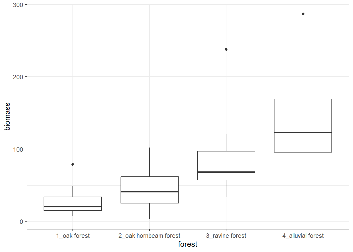
Alternatively, we can also do it like this, that we save the values to long format and use facet_wrap() to create more boxplots at once:
env %>%
  arrange(forest) %>%
  select(forest, cover_herbs = cov_herbs, biomass, cover_trees = cov_trees, soil_ph) %>%
  tidyr::pivot_longer(
    cols = c(cover_herbs, biomass, cover_trees, soil_ph),
    names_to = "variable",
    values_to = "value") %>%
  ggplot(aes(x = forest, y = value, fill = forest)) +
  geom_boxplot() +
  facet_wrap(~variable, scales = "free_y") +
  theme_bw() +
  theme(legend.position = 'none', axis.text.x = element_text(angle = 45, hjust = 1), axis.title = element_blank())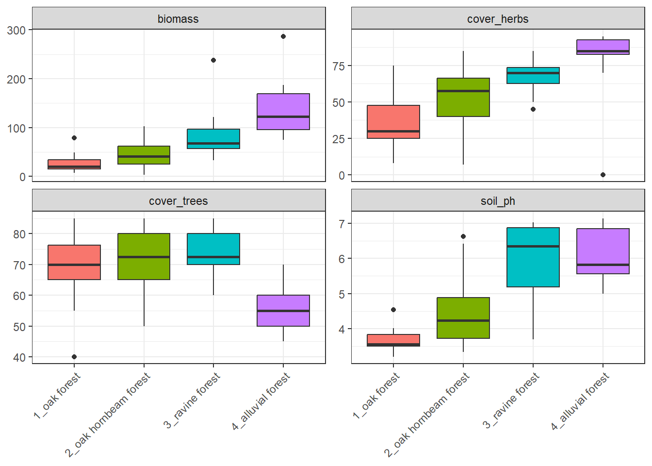
We might be interested in exploring the relationship between species richness and several factors. Below is an example of herb-layer species richness and biomass. At first, we need to calculate the species richness in the spe file. As an output, we want to plot this with different colours for different forest types, while keeping the regression line for the whole dataset.
spe %>%
  filter(layer %in% c(6, 7)) %>%
  count(releve_nr, name = "herblayer_richness") %>%
  left_join(env %>%
              select(releve_nr, biomass, forest), by = "releve_nr") %>%
  ggplot(aes(x = sqrt(biomass), y = herblayer_richness)) +
  geom_point(aes(colour = forest), size = 2, alpha = 0.8) +
  geom_smooth(method = "lm", se = TRUE, colour = "black") +
  theme_bw() +
  labs(
    x = "sqrt Biomass",
    y = "Herb-layer species richness",
    colour = "Forest type"
  )
`geom_smooth()` using formula = 'y ~ x'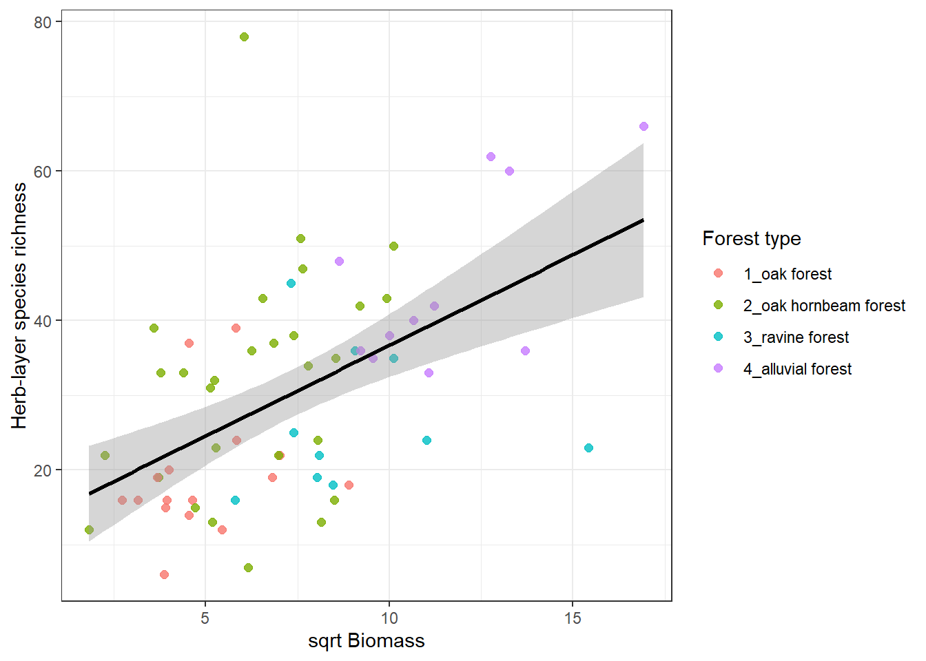
Boxplots of Ellenberg-type indicator values are based again on species data and values specific to each species. We will calculate the non-weighted mean for each plot and prepare boxplots for individual forest types. Again, we will use the step with long format and facet wrap.
spe %>%
  left_join(indicator_values) %>%
  select(-c(layer, cover_perc)) %>%
  distinct() %>%
  group_by(releve_nr) %>%
  summarise(across(starts_with("EIV"), ~mean(.x, na.rm = TRUE))) %>%
  left_join(env %>% select(releve_nr, forest)) %>%
  pivot_longer(
    cols = starts_with("EIV"),
    names_to = "EIV_variable",
    values_to = "value") %>%
  ggplot(aes(x = forest, y = value, fill = forest)) +
  geom_boxplot() +
  facet_wrap(~EIV_variable, scales = "free_y") +
  theme_bw() +
  theme(legend.position = 'none', axis.text.x = element_text(angle = 45, hjust = 1), axis.title = element_blank())
Joining with `by = join_by(species)`
Joining with `by = join_by(releve_nr)`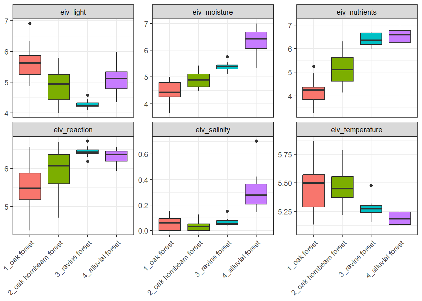
Proportions of endangered or alien species in forest types. We will first look at the numbers of these species, for example, the Red List (i.e., endangered) species. We would like to see the average number of Red List species per forest type.
env %>%
  select(releve_nr, forest) %>%
  left_join(spe %>%
              left_join(status) %>%
              filter(!is.na(redlist)) %>%
              count(releve_nr, name = "richness_redlist")) %>%
  left_join(spe %>%
              summarise(richness_all = n_distinct(species),
                        .by = releve_nr)) %>%
  mutate(richness_redlist = replace_na(richness_redlist, 0)) %>%
  mutate(richness_redlist_perc = richness_redlist/richness_all*100) %>%
  summarise(redlist_mean_perc = mean(richness_redlist_perc), .by = forest) %>%
  arrange(forest)
Joining with `by = join_by(species)`
Joining with `by = join_by(releve_nr)`
Joining with `by = join_by(releve_nr)`# A tibble: 4 × 2
forest redlist_mean_perc
<chr> <dbl>
1 1_oak forest 6.25
2 2_oak hornbeam forest 6.24
3 3_ravine forest 5.03
4 4_alluvial forest 1.71However, I can also examine the differences in the abundance of specific plant groups. What is the proportion of cover of alien species relative to total cover in different forests?
env %>%
  select(releve_nr, forest) %>%
  left_join(spe %>%
              left_join(status) %>%
              filter(origin %in% c("arch","neo")) %>%
              summarize(cover_alien = combine_cover(cover_perc),
                        .by = releve_nr))%>%
  left_join(spe %>%
              summarize(cover_total = combine_cover(cover_perc),
                        .by = releve_nr))%>%
  mutate(cover_alien = replace_na(cover_alien, 0)) %>%
  mutate(cover_alien_perc = cover_alien/cover_total*100) %>%
  summarise(alien_cover_mean_perc = mean(cover_alien_perc), .by = forest) %>%
  arrange(forest)
Joining with `by = join_by(species)`
Joining with `by = join_by(releve_nr)`
Joining with `by = join_by(releve_nr)`# A tibble: 4 × 2
forest alien_cover_mean_perc
<chr> <dbl>
1 1_oak forest 0.0188
2 2_oak hornbeam forest 1.24
3 3_ravine forest 3.11
4 4_alluvial forest 3.08 Almost at the end of this course!
A couple of tidyverse songs as a bonus for staying with us and learned many new things:
Human-made: https://www.youtube.com/watch?v=p8Py9C8iq2s
AI-made: https://suno.com/song/0599ca04-d17b-4fbd-8e3c-1a1a8a21e446?sh=iVMVs4IoyAXEoZMo
11.8 Exercises
These should be handed in to complete this course successfully.
Forest dataset from Turboveg database - prepare script from the database files as described above and (1) prepare scatterplot of a) overall species richness and b) herb-layer species richness against soil pH (2) scatterplot of herb-layer species richness against cover of trees (3) boxplots of richness (number of species) of native species, redlist species and alien species in individual forest types.
Use the data from the folder basiphilous_grasslands and recreate the following plot. Note that some data handling will be needed before you start plotting (transform the species abundance data from wide to long format, join species characteristics, calculate the number of species and number of specialists (
THE_THF) for each plot (Releve), join header data and transform the variable for the time of sampling (Rs_observ) to a character/factor).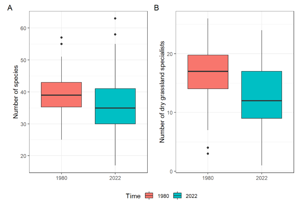
Frogs Use the data of the 10 most common frog species recorded within the Australian FrogID initiative. The original data comes from the TidyTuesdays repository, but we modified it slightly for this exercise and stored it in the
frogsfolder of our repository. The data are stored in multiple csv files, one for each species. Load all these files using a single pipeline (withmap()) and save to your environment as a single tibble >> prepare two barplots, first showing number of species in each stateProvince, and second showing number of all records irrespective of species >> prepare a table where there will be species as rows, columns for each stateProvince and values will represent the absolute number of records >> calculate also relative variables which will show representation of each species in the stateProvince relative to all species (%) in the stateProvince.Lepidoptera Work with this dataset, namely
spe_matrix_MSvejnoha, which is the species file with counts of moths in forest steppe localities. Import the data and check the structure >> count the number of all individuals at each site, i.e. abundance of moths >> from the env file import for each site, cover of herbs, shrubs, trees and dead wood >> prepare suitable graphs to visualise the relationship between abundance of moths and these variables characterising the vegetation.Acidophilous grasslands Import the head dataset, transform latitude and longitude into deg_lat and deg_long format >>prepare map with sites/sampled localities >> for vegetation types (
syntax_new) with more than 15 plots/samples prepare boxplots with comparison of species richness in old and new plots (information about new plots can be identified in the head as those sampled by M. Harásek, indicated as resampled).