Chapter 10: When assumptions are violated - data transformation and non-parametric methods

Log-normally distributed data

Log-normal distribution is very common in many kinds of biological data. These are random variables whose logarithm follows the normal distribution. As a result, log-normal variables may range from the zero limit (excluding zero itself) to plus infinity – that is pretty realistic e.g. for dimensions, mass, time, etc.

In contrast to the symmetric normal distribution, log-normal variables are positively skewed and display a positive correlation between mean and variance (Figure 1). A straightforward suggestion for such data is to apply log-transformation to the values to obtain normally distributed variables (Figures 1, 2, Table 1). ANOVA applied on non-transformed and transformed data provides quite different results (Table 1).

set.seed(42)

# create vector of jobs
jobs <- c("IT", "lawyer", "manager", "student")

# generate log-normally distributed data
it <- rlnorm(30, meanlog = 1.8, sdlog = 0.8)
lawyer <- rlnorm(35, meanlog = 2.1, sdlog = 0.7)
manager <- rlnorm(40, meanlog = 2.3, sdlog = 0.7)
student <- rlnorm(25, meanlog = 1.2, sdlog = 0.4)

# create data frame
calls <- data.frame(
  job = factor(rep(jobs, times = c(30, 35, 40, 25)), levels = jobs),
  length = c(it, lawyer, manager, student)
)

# plots
par(mfrow = c(1,2))
boxplot(length ~ job, data = calls)
boxplot(log(length) ~ job, data = calls)

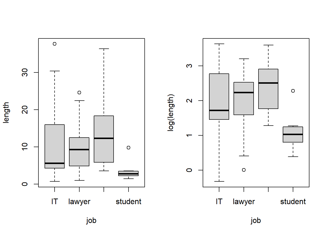
Figure 1: Example of a log-normal variable: effect of job on the length of phone calls. The left panel shows the boxplot on the ordinary linear scale, while the right panel shows the same values on the log-scaled y-axis.

par(mfrow = c(1,1))

The test may be then performed like this:

# anova not transformed
ntm <- lm(length ~ job, data = calls) # model
anova(ntm)             # test stats

Analysis of Variance Table

Response: length
           Df Sum Sq Mean Sq F value    Pr(>F)    
job         3 1657.4  552.48  11.196 1.455e-06 ***
Residuals 126 6217.8   49.35                      
---
Signif. codes:  0 '***' 0.001 '**' 0.01 '*' 0.05 '.' 0.1 ' ' 1

summary(ntm)$r.squared # r-squared

[1] 0.210463

# anova transformed
tm <- lm(log(length) ~ job, data = calls) # model
anova(tm)             # test stats

Analysis of Variance Table

Response: log(length)
           Df Sum Sq Mean Sq F value    Pr(>F)    
job         3 29.658  9.8860   18.93 3.379e-10 ***
Residuals 126 65.804  0.5223                      
---
Signif. codes:  0 '***' 0.001 '**' 0.01 '*' 0.05 '.' 0.1 ' ' 1

summary(tm)$r.squared # r-squared

[1] 0.3106795

Table 1: Summaries of ANOVA applied on non-transformed and transformed data displayed in Figure 1.

Analysis	\(R^2\)	\(F\)	\(DF\)	\(p\)
non-transformed	0.12	5.57	3, 126	0.00127
log-transformed	0.23	12.53	3, 126	3.15e-07

And these plots compare diagnostics plots of the transformed and non-transformed models:

par(mfrow = c(2,3))
plot(ntm, which = c(1,2,3))
plot(tm,  which = c(1,2,3))

Figure 2: Diagnostic plots of ANOVA models applied on non-transformed (upper row) and log-transformed data (lower row). Note the improved normal fit on the QQplot and homogeneity of variances after transformation (Residuals vs. Fitted and Scale-Location plots).

par(mfrow = c(1,1))

But log-transformation is not a simple utility procedure. It also affects the interpretation of the analysis. Log-transformation changes the scale from additive to multiplicative, i.e., we test the null hypothesis stating that the ratio between population means is 1 (instead of the difference being 0). We also consider different means – analysis on log-scale implies testing the geometric means on the original scale.

The same applies to regression coefficients, which become relative rather than absolute numbers, e.g., the slope indicates how many times the response variable will change with a change in the predictor. An example with log-transformation in linear regression is displayed in Figure 3, 4. and Table 2.

Log-transformation is sometimes used for data, which are not log-normally distributed but are just positively skewed. Such data may contain zeros and thus are not log-transformable. Instead log (x + constant) transformation must be used. Alternatively, square-root transformation may be considered for such data.

Note that the analysis results do not depend on the logarithm used – natural and decadic logarithms are used most frequently. Just beware of being consistent in using the same logarithm throughout the analysis.

set.seed(2468)

# generate fertilizer data
n <- 100
fertilizer <- runif(n, 5, 15)

# generate yield data (log normal)
log_yield <- 1.1 + 0.2 * fertilizer + rnorm(n, sd = 1.6)
yield <- exp(log_yield)

# data frame
maize <- data.frame(Fertilizer = fertilizer, Yield = yield)

# plot
par(mfrow = c(1,2))

### linear scale
plot(Yield ~ Fertilizer, data = maize,
     ylab = 'Grain yield')

### log scaled y-axis
plot(Yield ~ Fertilizer, data = maize,
     log = 'y',
     ylab = 'Grain yield')

Figure 3: Example of a regression with log-normal variable: how grain yield of maize depends on the amount of fertilizer applied. The left panel shows the scatterplot on the ordinary linear scale, while the right panel shows the same values on the log-scaled y-axis.

par(mfrow = c(1,1))

And this is how the tests would look like:

# anova not transformed
ntm2 <- lm(Yield ~ Fertilizer, data = maize) # model
anova(ntm2)             # test stats

Analysis of Variance Table

Response: Yield
           Df  Sum Sq Mean Sq F value  Pr(>F)  
Fertilizer  1  313920  313920  6.2491 0.01409 *
Residuals  98 4922942   50234                  
---
Signif. codes:  0 '***' 0.001 '**' 0.01 '*' 0.05 '.' 0.1 ' ' 1

summary(ntm2)$r.squared # r-squared

[1] 0.0599443

# anova transformed
tm2 <- lm(log(Yield) ~ Fertilizer, data = maize) # model
anova(tm2)             # test stats

Analysis of Variance Table

Response: log(Yield)
           Df  Sum Sq Mean Sq F value    Pr(>F)    
Fertilizer  1  30.851 30.8506  13.129 0.0004631 ***
Residuals  98 230.284  2.3498                      
---
Signif. codes:  0 '***' 0.001 '**' 0.01 '*' 0.05 '.' 0.1 ' ' 1

summary(tm2)$r.squared # r-squared

[1] 0.1181406

Table 2: ANOVA tables of linear models fitted on non-transformed and transformed data displayed in Figure 3.

Analysis	\(R^2\)	\(F\)	\(DF\)	\(p\)
non-transformed	0.06	6.28	1, 98	0.01386
log-transformed	0.11	11.52	1, 98	0.0009951

par(mfrow = c(2,4))
plot(ntm2, which = c(1,2,3,5))
plot(tm2,  which = c(1,2,3,5))

Figure 4: Diagnostic plots of linear models fitted on non-transformed (upper row of plots) and log-transformed data (lower row of plots). Note improved normal fit on the QQplot and improved homogeneity of variances after transformation (Scale-Location plot).

par(mfrow = c(1,1))

Non-parametric tests

Some distributions cannot be approximated by the normal distribution, and simple transformations may not be helpful. This applies to many data on the ordinal scale such as school grades, subjective rankings etc.

For such cases, non-parametric tests were developed (Table 3). These tests replace the original values by their order and use the resulting order values to test differences in central tendencies (which are not precisely means) between the samples. These tests are still based on the assumption that the samples come from the same, although not normal, distribution (which, however, is quite reasonable).

Table 3: List of parametric tests and their most common non-parametric counterparts together with appropriate R functions.

Parametric test	Non-parametric alternative	R function
two-sample t-test	Mann-Whitney U test	wilcox.test()
paired t-test	Wilcoxon test	wilcox.test() with parameter paired = T
one way ANOVA	Kruskal-Wallis test1	kruskal.test()
Pearson correlation	Spearman correlation	cor.test() with parameter method = 'spearman'

Permutation tests

Permutation tests represent valuable alternatives to parametric or non-parametric tests. First, a statistic of difference from the null hypothesis (between samples) is defined. That may be the raw or relative difference or an F-ratio if multiple groups are analyzed. This statistic is computed for observed data (observed statistic). Subsequently, values of the response variable are repeatedly permuted (reshuffled), and the same statistic is computed in each permutation. The p-value is then determined by the formula:

\[ p = \frac{x + 1}{n_{perm} + 1} \]

where \(x\) is the number of permutations in which test statistic was higher than observed test statistic, and \(n_{perm}\) is the total number of permutations.

NoteHow to do in R

1. Log-scaling of graph axes in ggplot2

• scale_y_continuous() - scaling of y axis

• scale_x_continuous() - scaling of x axis

• plus parameter trans = 'log10' to use decimal logarithm, trans = 'log2' to use 2 as the log-basis

• or you can use these handy wrapper functions: scale_y_log10() and scale_x_log10()

2. Log-transformation

• function log() for natural logarithm

• function log10() for decimal logarithm

3. Non-parametric tests

See Table 3.

4. Permutation tests

They are available in library coin:

• permutation-based ANOVA: oneway_test()

• permutation-based correlation: spearman_test()

Both functions require this parameter: distribution = approximate(B = number of permutations) to be set. B is usually set to 999 or 9999.

Exercises

1. Hair length was measured in two samples of twelve randomly chosen male students doing their studies at the faculty of science and the faculty of law.

   The measured hair length (in cm) was:

   Hair length of male students

   Faculty of science	Faculty of law
   14	6
   17	8
   29	2
   14	3
   14	4
   11	2
   39	10
   23	21
   18	5
   8	8
   51	3
   36	5

   Does the hair length of guys significantly differ depending on which faculty they do their studies?

2. The number of vascular plant species was recorded in 10 countries. How does the number of species depend on the country’s area?

3. Aggressiveness of football fans was monitored at 20 football matches of different leagues (0 = district league, 5 = Champions’ league) on an ordinal scale (0 = calm fans, 1 = loud support to players, 2 = loud support + some fireworks, 3 = loud support + many fireworks, 4 = fireworks thrown on the pitch, 5 = fans running on the pitch, 6 = fans running on the pitch and attacking the referee.

   The resulting data were as follows:

   Match ID	League	Aggressiveness
   1	2	0
   2	0	3
   3	2	4
   4	3	3
   5	4	0
   6	5	1
   7	2	3
   8	4	4
   9	2	4
   10	3	5
   11	4	0
   12	3	1
   13	2	4
   14	3	5
   15	1	5
   16	2	2
   17	1	4
   18	0	3
   19	5	2
   20	5	3

   Is the aggressiveness of fans associated with league level?

4. During the finals of the pizza tasting competition, ten evaluators tasted pairs of pizza samples prepared by cooks Francesco and Giacomo. Their evaluation (on a scale 1-5, 1 is best, 5 is worst) was the following. Is there any significant difference in the quality of pizza these guys make? Who will be the winner of the competition?

pizza <- data.frame(
  Francesco = c(1,2,1,1,3,1,1,2,1,2),
  Giacomo   = c(1,3,2,3,1,2,1,2,2,1)
  )

5. Lettuce varieties were evaluated for their taste. They also differed in leaf color. The taste was ranked on the scale (1 = delightful, 2 = very good, 3 = acceptable, 4 = bitter, not really good, 5 = ugly, disgusting). The resulting values are summarised here. Is there an association between leaf color and the taste of lettuce?

lettuce <- data.frame(
  red_leaved_varieties = c(1,2,1,2,1,2,2,1,1,1,3,1,1,3,1,3,1,3,3,2,2,3,1,2,3,1,1,4,1,2,2,2,2,2,2,1,2,3,1,1,2,2,2,2,2,2,1,1,2,2,3,1,2,1,1,2,2,1,1,2),
  green_leaved_varieties = c(4,2,2,1,2,2,1,3,2,1,2,4,3,3,3,3,2,3,2,1,4,2,2,3,2,2,1,1,5,3,3,2,3,2,1,3,3,2,2,1,2,2,3,3,3,1,1,3,2,3,3,3,2,1,2,3,2,2,3,1)
)

6. 24 people read 24 books (one each) written by four different authors (6 by each). After reading the book, they were asked to rate the book on a scale: 1 – annoying, 2 – boring, 3 – mostly boring with some enjoyable parts, 4 – enjoyable, and 5 – wonderful.

   The resulting data are summarised below:

   Book ratings

   Ernest Hemingway	Charles Dickens	Alexander Pushkin	Lev Tolstoy
   4	2	3	2
   5	4	4	1
   4	5	5	3
   4	5	4	2
   3	2	3	3
   4	4	3	2

   Is there any significant difference in rating among these authors? Which of them has the highest average rating?

Real data tasks

7. Analyse the relationship between three types (the variable Type) of plant Odontites vernus defined on ploidy level (2n = 2x and 2n = 4x) and time of flowering (early = June and late = August), and morphology of the plants quantified by the number of internodes (the variable Internodes_total). Tests if the three types of the species differ in the internode number. Consider how the data align with the assumptions of ANOVA, and if not, find a suitable solution. The data are available from data/Odontites_cytotypes_morphology.xlsx. The original publication is available here.

8. Analyse the dependence between vegetation species richness (number of species) and plant-available phosphorus concentration in the soil in the dataset of vegetation plots of Latvian grasslands. Consider how the data align with the assumptions of linear regression, and if not, find a suitable solution. The data are available from data/LatviaGrasslands.xlsx. The data come from the master thesis of Martin Franc (in Czech with English abstract).

#AI Ask your favourite LLM to solve any of the tasks and generate the corresponding R script. Discuss with the LLM possible transformations and uses of different non-parametric tests.

Footnotes

1. In this case, Dunn test may be used for post-hoc comparisons (function dunnTest() in package FSA).